1. Quarterly earnings
The data for this assignment are listed in the Excel file Quarterly earnings.
The quarterly earnings (in millions of dollars) of a large soft-drink manufacturer have been recorded for the years 2007 to 2010. The manufacturer wants to forecast the quarterly earnings for the years 2011 and 2012 based on the regression line 
 .
.
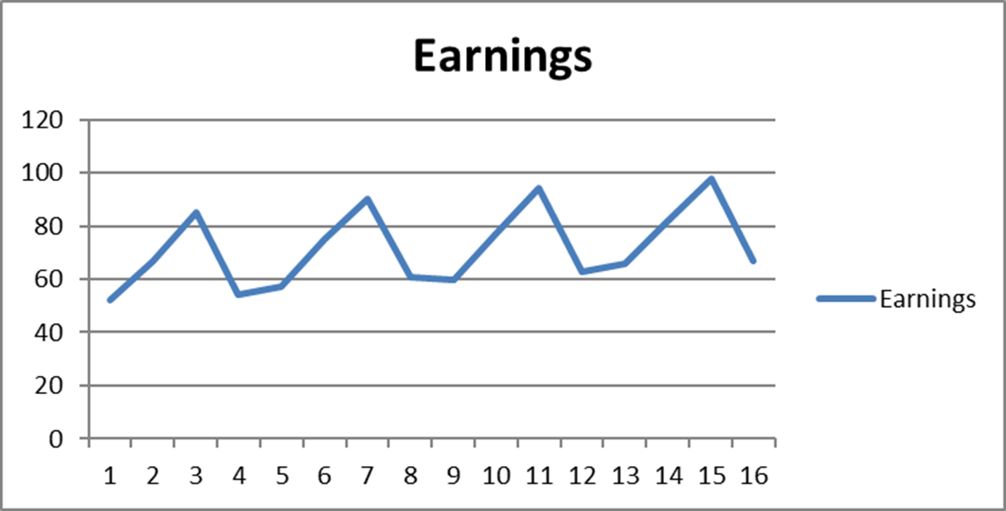
a. How can you demonstrate that the earnings show seasonal variation? Give a rough sketch of the earnings.
b. How well does the model fit the data? Consider the coefficient of determination, the -value of the -test and the -value of the coefficient of time. Why is the coefficient of determination of less importance in this case?
c. Explain briefly in words what seasonal indexes are. How can you compute these?
d. The seasonal indexes are 0.893; 1.058; 1.270; 0.833. Now the manufacturer can use the seasonal indexes in combination with the regression equation to forecast the earnings for the years 2011 to 2012. Show that the forecasts are (just take the first three): ;
;  ;
;  ;
;  ;
;  ;
;  ;
;  ;
; 
Solution.
a. If you plot the earnings you find as a result a jigsaw graph repeating itself after 4 periods, with a slightly positive trend. This demonstrates the presence of seasonal variation.
b. The model fits poorly since the coefficient of determination is too low  : . The
  -value of
  is too high: 0.1403 and also the -value of Period is too high. The low coefficient of determination is less relevant because we are only interested in a trend line.
c. Based on the regression values  and the observed values
  , for all quarters the ratio
  is computed. For each quarter the mean of these ratios, the seasonal indexes, is computed.
These indexes tell us that the Q1 earnings are 16% below the Q1 average; the Q2 earnings are 6% above the Q2 average etc.
d.  ;
;  ;
;  ;
;  .
.
The forecasts are based on the formula  . For
. For  is taken the value that is related to the corresponding quarter, so: