Time series – seasons

A variable measured over time (in sequential order) is called a time series. From this data, we analyze it to detect patterns that will enable us to forecast future values of the variable. This technique has wide application:

Governments want to know future values of interest rates, unemployment rates and percentage increases in the cost of living;
Housing industry economists must forecast mortgage interest rates, demand for housing, and the cost of building materials;
Many companies attempt to predict the demand for their product and their share of the market;
Universities and colleges often try to forecast the number of students who will be applying for acceptance at post-secondary-school institutions.

Time series components

A time series can consist of four different components:

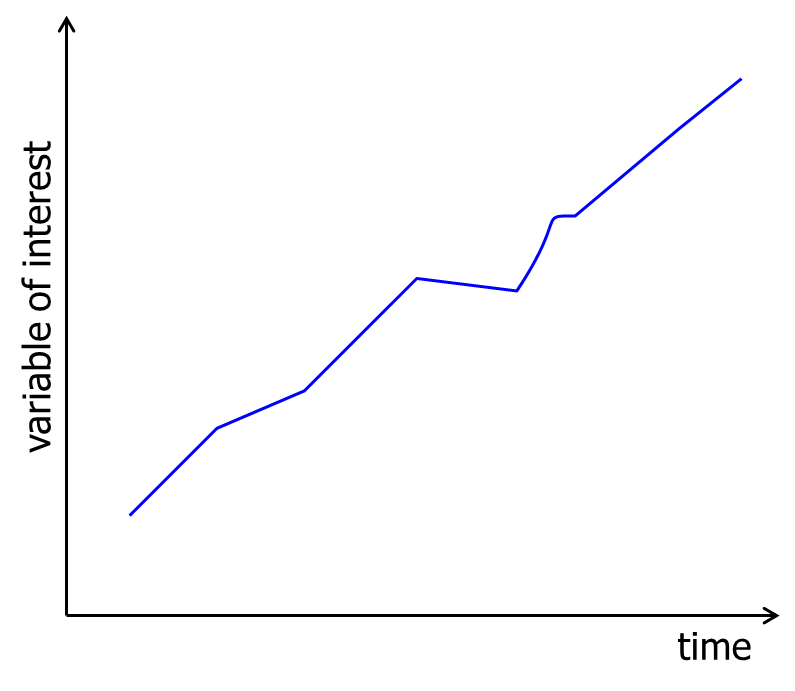
Long-term trend
This is a long term relatively smooth pattern or direction, that persists usually for more than one year. An example is the world population.

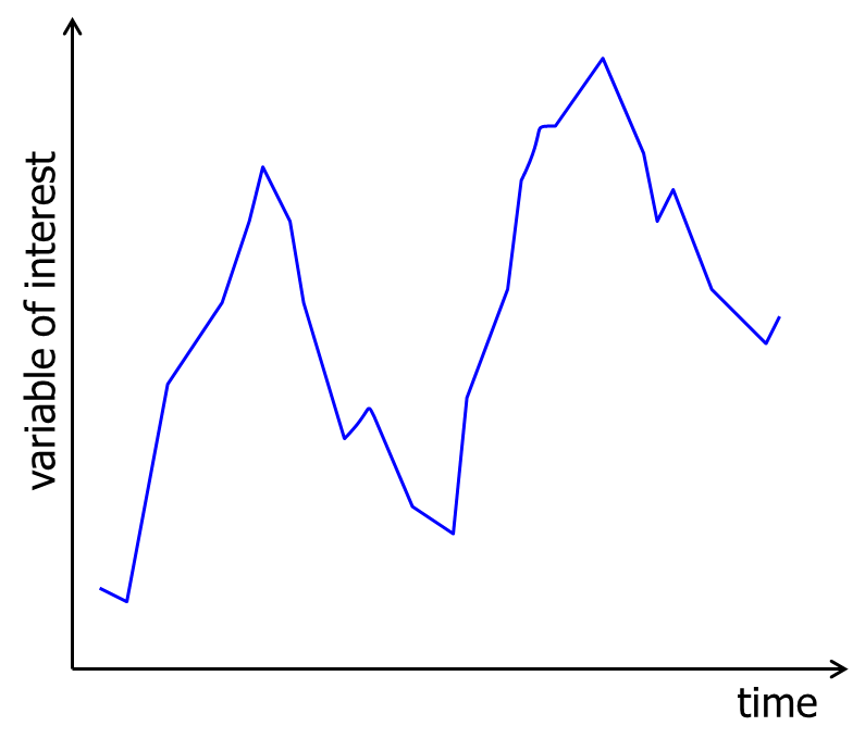
Cyclical variation
A cycle is a wavelike pattern describing a long term behavior(for more than one year). An example are house prices. Cyclical patterns that are consistent and predictable are quite rare; hence, we will ignore this type of variation.

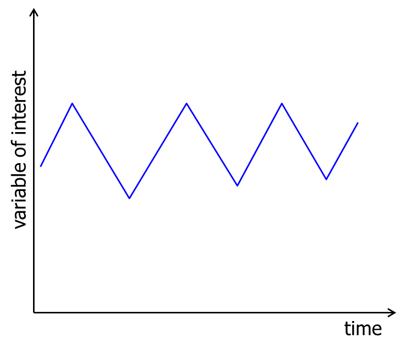
Seasonal variation
The seasonal component of the time series exhibits a short term (less than one year) calendar repetitive behavior. Examples are the number of guests in a restaurant (week) and a hotel occupancy rate (quarter).

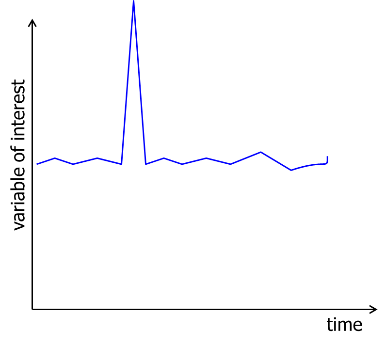
Random variation
Random variation comprises the irregular unpredictable changes in the time series. It tends to hide the other (more predictable) components. One of our objectives will be to remove random variation.

Trend and seasonal effects

We are particularly interested in the seasonal effects or seasonal variation, especially in the underlying trend. A trend can be linear or nonlinear. The easiest way of measuring the long-term trend is by regression analysis, where the independent variable is time.

Seasonal analysis

Seasonal variation may occur within a year or within shorter intervals, such as a quarter, month, week, or day (e.g. hotel occupancy: quarter; consumer spendings: month; restaurant: week; call center: hour). To measure the seasonal effect, we compute seasonal indexes, which gauge the degree to which the seasons differ from one another.
In the following we have two aims:

We want to eliminate the seasonal variation as much as possible so that we get a clear view on the actual underlying trend. This process is also known as 'deseasonalizing';
Based on the data we want to generate an accurate forecast for the coming periods.

The following prodedure can be used to compute the so-called seasonal indexes.

Compute the sample regression line $\hat{y}_t=b_0+b_1x_1$ which can be considered as a trend line;
For each time period, compute the ratio: $\displaystyle{\frac{y_t}{\hat{y}_t}}$ . This ratio is a measure of how much the actual observations are above or below the trendline and define the seasonal effects;
For each type of season, compute the average of the ratios from step 2.

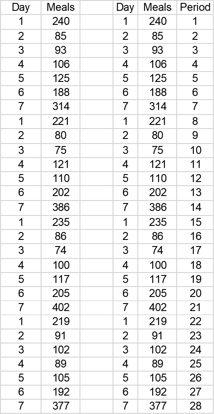
In the following example a take away restaurant registered the daily number of ordered meals during 4 weeks. The two columns at the left show the original data. Since a time series analysis cannot be performed with the Days column, we add an extra column Period containing 28 periods.

Linear regression is used to produce the trend over 4 weeks and gives the following regression equation:

$\hat{y}=145.23+1.66$ Period

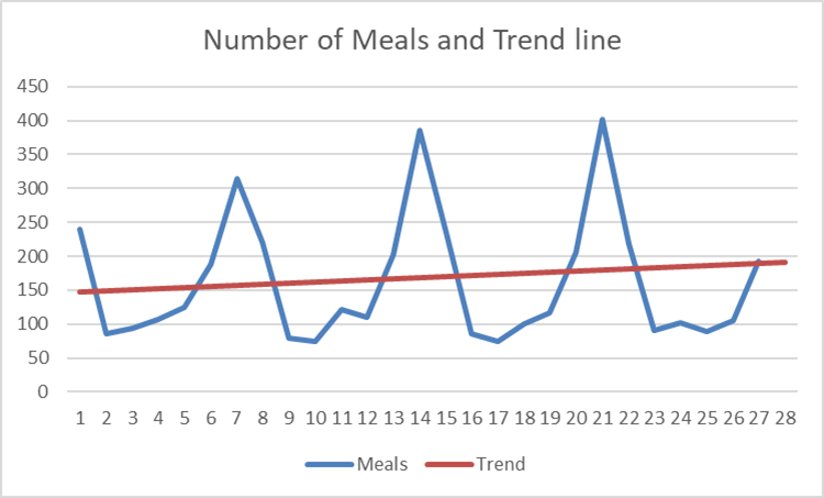
The observations show that the number of meals are (very) large for some periods ( $\displaystyle{\frac{y_t}{\hat{y}_t}>1}$ , periods 7, 14, 21. 28, i.e. Saturdays) and much less $\displaystyle{\frac{y_t}{\hat{y}_t}<1}$ for the periods 2, 9, 16, 23, i.e. Mondays) which are 'seasonal' effects: more meals at the end of the week and less during the week.

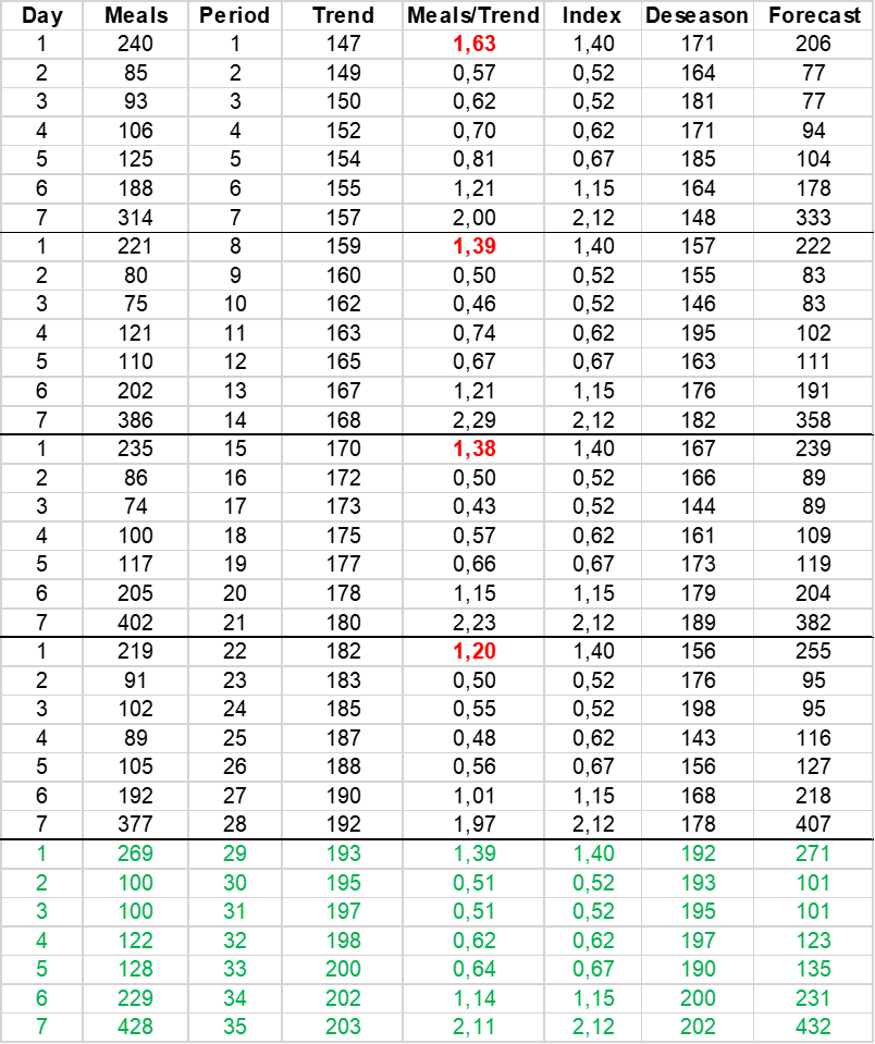
In the following table the columns Day, Meals and Period are extended by the regression output $\hat{y}$ , the ratio $y/\hat{y}$ , Index and Adjusted. Black numbers refer to the periods $1, \cdots,28$ , the green numbers represent forecasting computations (periods $29,\cdots,25$ .
For each period the ratio $y/\hat{y}$ is computed. When the number of meals is above the daily average, this variable will be $>1$ . When the number of meals is below the daily average, the variable will be $<1$ . The Index is the mean of these values for each period. For example, for the periods 1, 8, 15, 22 the variable $y/\hat{y}=1.63;1.39;1.38$ and $1.20$ . The mean of these numbers is $1.40$ which is called the Index of the periods 1, 8, 15 and 22. In fact, this number expresses that on average on these days about 1.40 times more meals are ordered than the regression line indicates.
Period 3 on the other hand has an Index $=0.52$ suggesting that on these days the revenue is about half of the number the regression line indicates.

The results are found in the following table.

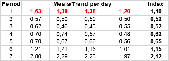
The seasonal indexes tell us that, on average, the number of ordered meals on days $2,\cdots,5$ are below the average, and on the other days above the average.

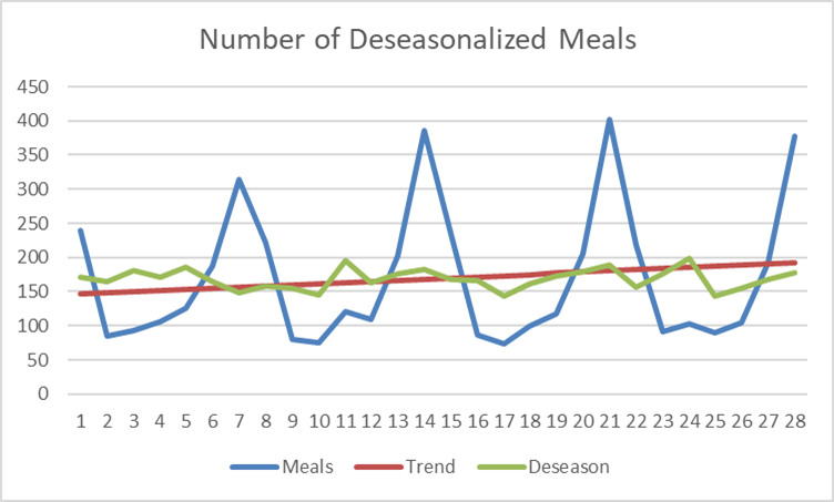
One application of seasonal indexes is to remove the seasonal variation in a time series, by deseasonalizing. In the figure below we find the original ordered meals (Meals), the trend line and the deseasonalized data (Meals/Index).

Forecasting

We want to calculate a forecast $F(t)$ for days $29,\cdots,35$ . We use the trend line as a basis for these computations and multiply the trend line by the Index, so $F(t)=(b_0+b_1t)$ Index. When we apply this formula to the original data, we see a small difference with the original data on those days (1, …,28 ). This difference occurs because $y/\hat{y}$ is not used per period, but their average over the four periods. The result can be seen in the figure below.

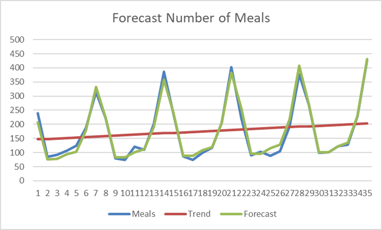
The forecasted ordered meals on day $29,\cdots,35$ are $271, 101, 101, 123, 135, 231, 432$ .