Estimation

The objective of estimation is to estimate the value of a population parameter based on a sample statistic. E.g., the sample mean $\overline_{X}$ is employed to estimate the population mean $\mu$ . Unfortunately, $\overline_{X}$ is almost always unequal to $\mu$ . So, then what is the use of $\overline_{X}$ ?

Two types of estimators

1. Point estimator

A point estimator is a number such as $\overline{X}$ . We use this number because we hope that it will be equal to the unknown population parameter $\mu$ .
However, in continuous distributions the probability that this will be the case is virtually zero. Hence we will employ the interval estimator to estimate population parameters.

2. Interval estimator

An interval estimator draws inferences about a population by estimating the value of an unknown parameter using an interval. That is, we say (with some certainty) that the population parameter of interest is between some lower and upper bounds.
We have the following 3 characteristics of estimators:

An unbiased estimator of a population parameter is an estimator whose expected value is equal to that parameter (e.g. $E(\overline{X})=\mu$ ; $E(s^2)=\sigma^2$ ;
An unbiased estimator is said to be consistent if the difference between the estimator and the parameter grows smaller as the sample size grows larger;
If there are two unbiased estimators of a parameter, the one whose variance is smaller is said to be relatively efficient.

Unbiased estimators

The sample mean $\overline{X}$ and the sample variance $s^2$ are unbiased estimators, because their expected values equal the population mean and variance $\mu$ and $\sigma^2$ :

$\displaystyle{E(\overline{X} )=E(\frac{1}{n}\sum{}{}X)=\frac{1}{n}\sum{}{}E(X)=\frac{1}{n}\sum{}{}\mu=\frac{1}{n}n\mu=\mu}$

Similarly, we find (a little more difficult to prove):

$E(s^2 )=\sigma^2$ (if the denominator of $s^2$ is taken equal to n-1).

For a symmetric distribution the median is an unbiased estimator since $E($ sample median $)=\mu$ .

Consistency

An unbiased estimator is said to be consistent if the difference between the estimator and the parameter grows smaller as the sample size grows larger.

E.g. $\overline{X}$ is a consistent estimator of $\mu$ because:

$\displaystyle{V(\overline{X})=\sigma^2/n}$ and $\displaystyle{\lim_{n \to \infty} V(\overline{X})=0}$

And thus, as $n$ grows larger, the variance of $\overline{X}$ grows smaller.

For a symmetric distribution the sample median is also a consistent estimator of $\mu$ because:

$V($ sample median $)= 1.57\sigma^2/n$ (Mathematics!)

And thus, as $n$ grows larger, the variance of the sample median grows smaller.

Estimating the mean (known population variance)

In Chapter 8 we produced the following general probability statement about $\overline{X}$ .

$\displaystyle{P(-Z_{\alpha/2}<Z<+Z_{\alpha/2})=1-\alpha}$

$\displaystyle{Z=\frac{\overline{X}-\mu_{\overline{X}}}{\sigma_{\overline{X}}}=\displaystyle{\frac{\overline{X}-\mu_X}{\sigma_{X}/\sqrt{n}}}$

$Z$ is (approximately) standard normally distributed (also consider the Central Limit Theorem).

$\alpha$ is the significance level: the proportion of times that an estimating procedure will be wrong.

$1-\alpha$ is the confidence level: the proportion of times that an estimating procedure will be correct.

So,

$\dispaystyle{P(-Z_{\alpha/2}<\frac{\overline{X}-\mu}{\sigma/\sqrt{n}}<+Z_{\alpha/2})=1-\alpha}$

After some algebra we get the following confidence interval estimate of $\mu$ .

$\displaystyle{P(\overline{X}-Z_{\alpha/2}\frac{\sigma}{\sqrt{n}}<\mu<\overline{X}+Z_{\alpha/2}\frac{\sigma}{\sqrt{n}})=1-\alpha}$

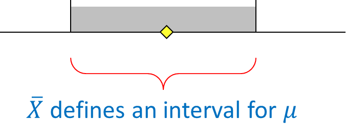
If the significance level is $\alph=0.05$ or $5$ % then we speak of the 95% confidence interval estimate. This formula is a probability statement about $\overline{X}$ : this statistic defines an interval containing $\mu$ with confidence $1-\alpha$ .

Example
Given the following sample of 25 observations of a normally distributed population:

235, 421, 394, 261, 386, 374, 361, 439, 374, 316, 309, 514, 348, 302, 296, 499, 462, 344, 466, 332, 253, 369, 330, 535, 334

Then what is the $95$ % confidence interval of $\mu$ if $\sigma=75$ ?

First, the Anderson-Darling test shows that the data are normally distributed ( $A=0.32462, p=0.5066)$ and then the formula for the confidence interval is valid.

Using Excel we find that he mean is $370.16$ and the $95$ % interval is $[340.76. 399.56]$ .

Interpreting the interval estimator

The confidence interval should be interpreted as follows.
It states that there is a ( $1-\alpha$ ) probability that the interval will include the population mean. Once the sample mean is computed, the interval shows the lower and upper limits of the interval estimate of the population mean.

Example
We computed earlier that a fair dice has a population mean $\mu=3.5$ and a population standard deviation $\sigma=1.71$ . Suppose we don’t know the mean and construct the $90$ % confidence interval $\overline{X} \pm 2.81$ based on a sample of size $100$ .

$\displaystyle{Z_{0.05}{\frac{\sigma}{\sqrt{n}}=1.645{\frac{1.71}{10}=2.81)}$

Next we repeat this sample 40 times, compute $\overline{X}$ each time and get a confidence interval. There is a 90% probability that this value of $\overline{X}$ will be such that $\mu$ would lie somewhere between $\overline{X}-2.81$ and $\overline{X}+2.81$ .

Table 10.2 (p. 334-347) in Keller shows that we expect that in about 4 of the 40 cases (10%) the confidence interval will not include the value $3.5$ (accidentally, in this example exactly 4 cases).

Interval bound

The bound $B$ of a confidence interval is a function of the significance level, the population standard deviation and the sample size:

$\displaystyle{B=Z_{\alpha/2}{\frac{\sigma}{\sqrt{n}}}$

so that the confidence interval is

$[\mu-B, \mu+B]$

A smaller significance level α (e.g. $1$ % instead of $5$ %) gives a larger value of $Z_{\alpha/2}$ , and a larger confidence ( $99$ % vs. $95$ %) and thus a wider confidence interval, so less accurate information.

Larger values of $\sigma$ produce wider confidence intervals, so less accurate information.

Increasing the sample size $n$ decreases the bound of the confidence interval while the confidence level can remain unchanged, so more accurate information.

Selecting the sample size

Earlier we pointed out that a sampling error is the difference between an estimator and a parameter. We can also define this difference as the error of estimation. This can be expressed as the difference between $\overline{X}$ and $\mu$ .

From the formula for the bound we can easily derive:

$\displaystyle{n=(\frac{Z_{\alpha/2}\sigma}{B}})^2}$

If a given $B$ is required, just compute the corresponding sample size $n$ .

Estimating the mean (unknown population variance)

In practice, the population standard deviation $\sigma$ is unknown. Then its estimate, the sample standard deviation $s$ , is taken instead.

However, $\displaystyle{\frac{\overline{X}-\mu}{s/\sqrt{n}}}$ has no standard normal distribution (a ratio of two random variables), but we approximate:

$\displaystyle{t_{n-1}\approx\frac{\overline{X}-\mu}{s/\sqrt{n}}}$

The Student’s $t_n$ distribution approximates the Z-distribution for larger $n$ : $\displaystyle{\lim_{n \to \infty} t_n=Z}$ .

Now the corresponding $1-\alpha$ confidence interval will be:

$\displaystyle{P(\overline{X}-t_{n-1,\alpha/2}\frac{s}{\sqrt{n}}<\mu<\overline{X}+t_{n-1,\alpha/2}\frac{s}{\sqrt{n}})=1-\alpha}$

$n-1$ is called the degrees of freedom (we write $df$ or $\nu$ ), thus the sample size minus $1$ .

The normality condition for $X$ is required but for larger $n$ the Central Limit Theorem will hold: for larger $n$ the sample mean $\overline{X}$ will be approximately normal.

Example
What is the $95$ % confidence interval of $\mu$ for the following set of data, if $\sigma$ is unknown.

235, 421, 394, 261, 386, 374, 361, 439, 374, 316, 309, 514, 348, 302, 296, 499, 462, 344, 466, 332, 253, 369, 330, 535, 334

We can use the confidence interval but Excel can do the job as well. The confidence interval will be $[336.81, 403.51]$ .

Estimation

Estimation

Two types of estimators

Unbiased estimators

Consistency

Estimating the mean (known population variance)

Interpreting the interval estimator

Interval bound

Selecting the sample size

Estimating the mean (unknown population variance)

Contact

Tutor Math, Statistics or GMAT?

Language preference