The basics of Statistics

(Keller 4-1, 2, 3, 4)

Population vs. Sample

A population consists of all objects of interest (e.g. all students at Erasmus University Rotterdam, approximately 35000 students). Usually the number of objects in a population is denoted as $N$ , the population size).

A sample consists of a (random) selection from the population. For instance 100 students taken from all students at Erasmus University Rotterdam. Usually the number of objects in a sample is denoted as ( $n$ ≪ $N$ ), the sample size.

Data types

The following data types are defined:

Nominal / Categorical (text, no order, e.g. capital city: "Amsterdam", "Paris", "Bordeaux");
Ordinal (nominal with some order, e.g. army ranks: "General", "Corporal", "Private");
Interval (real numbers, e.g. profit: $2.1$ %);
Ratio (interval with true zero point, e.g. weight: 80 kg).

Often the ratio type is not used, as is the case in the Keller book.

Numerical descriptive statistics

The most important descriptive statistics are the following:

Measures of central location, e.g. mean, median, mode;
Measures of variability, e.g. variance, standard deviation, range, coefficient of variation;
Measures of relative standing, e.g. percentiles, Quartiles ( $Q_1, Q_2, Q_3)$ , Interquartile Range $IQR= Q_3-Q_1$ ;
Graphical representation of data, e.g. boxplots, histograms;
Measures of linear relationship, e.g. covariance, correlation, determination, regression equation.

Measures of central location

The following measures of central location are used.

The arithmetic mean, also known as average, shortened to mean, is the most popular and useful measure of central location.
It is computed by simply adding up all the (numerical) obervations and dividing the sum by the total number of observations $x_i$ ;
The population mean is $\displaystyle{\mu=\frac{\sum_{}{}x_i}{N}$ , $i=1,\cdots,N}$ ;
The sample mean is $\displaystyle{\overline{x}=\frac{\sum_{}{}x_i}{n}$ , $i=1,\cdots,n}$ .

The arithmetic mean

The arithmetic mean is appropriate for describing interval data, e.g. heights of people, marks of students, prices, etc.;
A disadventage is that it is seriously affected by extreme values called outliers. E.g. if one observation is much larger than usual (by a typo), such as 579990 in the following observations: $45, 76, 38, 55, 579999, 16, 44$ .

The median

The median is calculated by placing all observations in increasing order; the observation that falls in the middle is the median.

Example
Data: $0, 7, 12, 5, 14, 8, 0, 9, 22$ (uneven, so there is a middle number);
Sort them from bottom to top, and find the middle;
$0, 0, 5, 7, 8, 9, 12, 14, 22$ - The median is: $8$ .

Example
Data: $0, 7, 12, 5, 14, 8, 0, 9, 22, 33$ (even);
Sort them from botton to top, and find the middle by averaging both middle numbers;
$0, 0, 5, 7, 8, 9, 12, 14, 22, 33$ The median is $\displaystyle{\frac{(8+9)}{2}=8.5}$ .

The mode

The mode of a set of observations is the value that occurs most frequently. For example, of a number of international students, which nationality occurs most often?
If 10 students have the following nationalities: France, France, USA, China, Netherlands, France, China, France, Spain. Italy, then the mode is France.
A set of data may also have two, or more modes.
The mode can be used for all data types, though it is mainly used for nominal data.

Which is the best, mean or median?

The mean is used most frequently.

Example
$0, 7, 12, 5, 14, 8, 0, 9, 22, 33$
The mean $= 11.0$ and the median $= 8.5$ .

Now suppose that the respondent who reported $33$ actually reported $333$ (a typo). The mean changes sharply but the median does not change.

$0, 7, 12, 5, 14, 8, 0, 9, 22, 333$
The mean $= 41.0$ (instead of $11.0$ ) and the median remains $= 8.5$ .

So, the median is less sensitive for outliers.

Measures of variability

There are several possible measures of variability, but why don't we just take the mean of the deviations from the mean as a measure of the spread? Unfortunately, this will always be zero: $(\sum{}{}(x_i-\mu)= \sum{}{}x_i-\sum{}{}\mu=n\mu -n\mu=0$ ).

Then, why not take the absolute value of the deviations from the mean: $\sum{}{}|x_i-\mu|/N$ ? This would be possible but absolute value functions are difficult to handle mathematically.

Other possible measures are:
Range = max - min of the data;
Interquartile range IQR = $Q_3 - Q_1$ . For the explanations of quartiles see later.

The variance is the mean squared deviations from the mean. Although this measure is not exactly what we want, it is used frequently and successfully in Statistics.

Variance and standard deviation

The variance and its related measure standard deviation, are most important measures in Statistics. They play a vital role in almost all statistical inference procedures.
The population variance is denoted by $\sigma^2$ and the population standard deviation is $\sigma=\sqrt{\sigma^2}$ .
The sample variance is denoted by $s^2$ and the sample standard deviation is $s=\sqrt{s^2}$ .
The population variance is: $\displaystyle{\sigma^2=\frac{\sum{}{}(x_i-\mu)^2}{N}}$ , $N$ is the population size.
The sample variance is: $\displaystyle{s^2=\frac{\sum{}{}(x_i-\overline{x})^2}{n-1}}$ , $n$ is the sample size.
$n-1$ is called the degrees of freedom (df).

Interpreting the standard deviation

The standard deviation is used to compare the variability of a distribution and make a statement about the general shape of a distribution. If the histogram is bell-shaped, we can use the Empirical rule:

Approximately 68% of all observations fall within one standard deviation of the mean;
Approximately 95% of all observations fall within two standard deviations of the mean;
Approximately 99.7% of all observations fall within three standard deviations of the mean.

If the distribution is normal, then these percentages are exact.

Range

The range of a set of interval data is the difference between the largest and smallest observation.

Example
Data set: $7, 7, 12, 5, 14, 8, 22, 9, 20$
The difference is $22-5=7$

Measures of relative standing

Measures of relative standing are designed to provide information about the position of particular values relative to the entire data set.

Percentile: the $p^{th}$ percentile is the value for which $p$ % are less than that value and $(100-p)$ % are greater than that value.

Example
Suppose you scored in the $60^{th}$ percentile on an exam. This means that 60% of the other scores were below yours, while 40% of the scores were above yours.

Quartiles

There are special names for the $25^{th}$ , $50^{th}$ , $75^{th}$ percentile, named quartiles.

The first or lower quartile is labeled $Q_1= 25^{th}$ percentile;
The second quartile is $Q_2= 50^{th}$ percentile (the median);
The third or upper quartile is labeled $Q_3= 75^{th}$ percentile.

Interquartile range (IQR)

The quartiles can be used to create one more measure of variability, the interquartile range (IQR), which is defined as follows:

Interquartile range IQR $=Q_3- Q_1$

The interquartile range measures the spread of the middle $50$ % of the observations. Large values of this statistic means that the $1^{st}$ and $3^{rd}$ quartiles are far apart indicating a high level of variability.

Example
IQR $(7, 7, 12, 5, 14, 8, 22, 9, 20)=8.5$ , according to Excel.

Boxplots and histograms

The boxplot is a technique that graphs a number of statistics, such as $Q_1, Q_2$ (median), $Q_3$ , ICR and outliers.

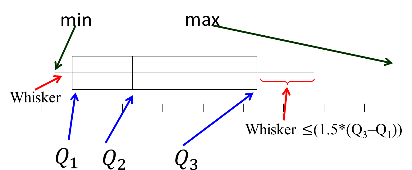
The horizontal lines extending to the left and right are called whiskers. Any points that lie outside the whiskers are called outliers. The whiskers extend outward to the smaller of 1.5 times the interquartile range or to the most extreme point that is not an outlier.

The following boxplots compare a number of US hamburger chains.

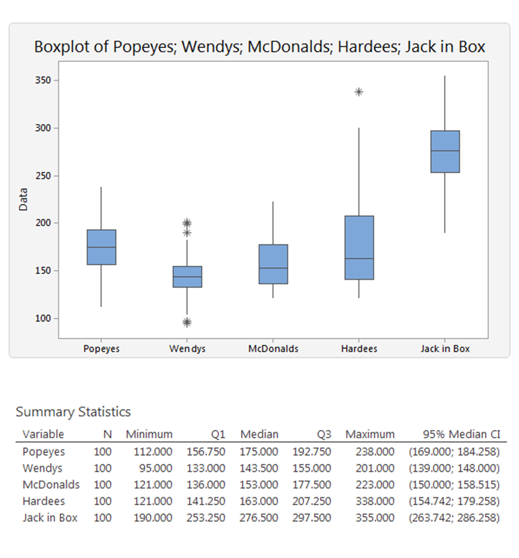
These hamburger chains are compared with respect to their service times. Wendy’s service time is shortest and least variable. Hardee’s has the greatest variability, while Jack-in-the-Box has the longest service times.

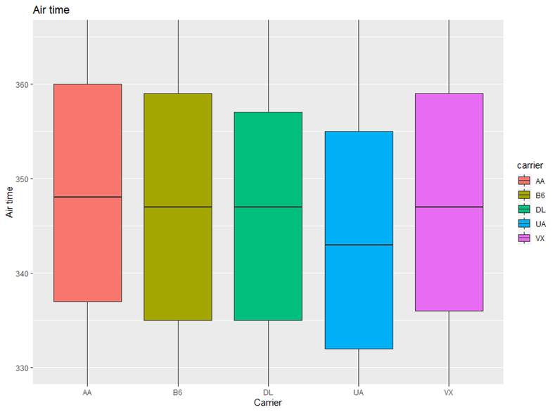
The following graph shows the boxplots of air time of 5 carriers flying from JFK to SFO. UA has the smallest median. the variability is almost the same.

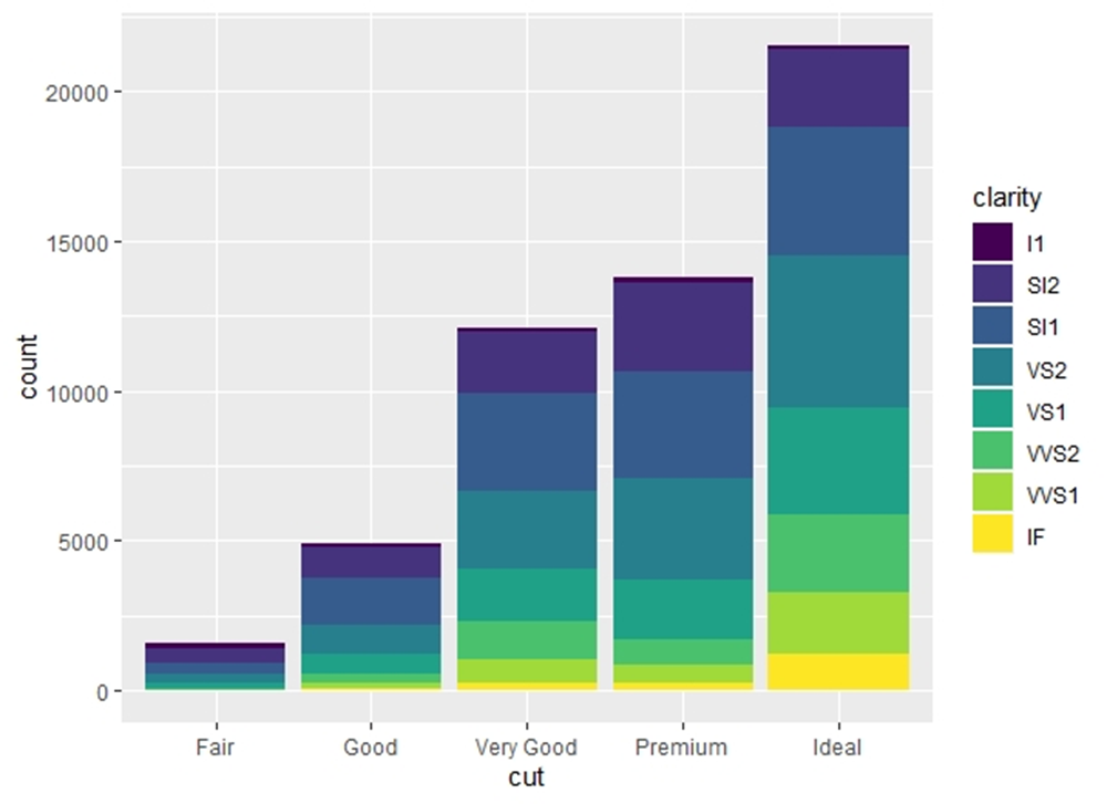
The following graphs (made by the programming language R and using the large data set Diamonds) show the distribution of the clarity of the various types of quality of diamonds. This data set contains about 22000 'ideal' cut diamonds, most of them have a clarity VS2 and only a few hundred clarity IF.

Measures of linear relationship

There are three numerical measures of linear relationship that provide information as to the strength and direction (positive / negative) of a linear relationship between two variables (if one exists).

Covariance;
Coefficient of correlation;
Coefficient of determination.

Covariance

The population covariance between two variables $X$ and $Y$ is defined as follows ( $N$ is the population size):

$\displaystyle{\sigma_{xy}=\frac{\sum{}{}(x_i-\mu_x)(y_i-\mu_y)}{N}}$

The sample covariance between the variables $X$ and $Y$ is defined as follows ( $n$ is the sample size):

$\displaystyle{s_{xy}=\frac{\sum_{}{}(x_i-\overline{x})(y_i-\overline{y})}{n-1}}$

Example
The table below shows two samples $X$ and $Y$ .

In each set the values of $X$ are the same and the values of $Y$ are the same; the only thing that has changed is the order of the $Y$ ’s.

In Set 1: as $X$ increases, so does $Y$ : $s_{xy}$ is large and positive;
In Set 2: as $X$ increases, $Y$ decreases: $s_{xy}$ is large and negative;
In Set 3: as $X$ increases, $Y$ does not in any particular way: $\displaystyle{s_{xy}}$ is small (close to 0).

In general we note:

When two variables move in the same direction (both increase or decrease), the covariance is a ‘large’ positive number;
When two variables move in opposite direction, the covariance is a ‘large’ negative number;
When there is no particular pattern, the covariance is a ‘small’ number (close to 0).

However, what is large or and what is small?

Coefficient of correlation

The covariance has a disadvantage, it has not limited. A larger covariance in one situation does not mean a stronger relationship than a smaller covariance in another relationship. The coefficient of correlation solves this problem: it lies in the interval $[-1,+1]$ . It is defined as the covariance divided by the standard deviations of the variables.

The population coefficient of correlation is:

$\displaystyle{\rho=\frac{\sigma_{xy}}{\sigma_{x}\sigma_{y}}}$

The sample coefficient of correlation is:

$\displaystyle{r=\frac{s_{xy}}{s_{x}s_{y}}}$

The coefficient of correlation answers the question: how strong is the association between $X$ and $Y$ ?

The advantage of the coefficient of correlation over the covariance is that it has a fixed range from $-1$ to $+1$ (proven by Mathematics). If the two variables are very strongly and positively related, the coefficient value is close to $+1$ (strong positive linear relationship). If the two variables are very strongly and negatively related, the coefficient value is close to $-1$ (strong negative linear relationship). No straight linear relationship is indicated by a coefficient close to 0.
The following graphs depict the relations of $X$ and $Y$ for various coefficients of correlation, varying from $-1$ to $+1$ .

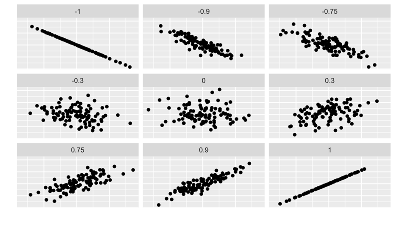
We can judge the coefficient of correlation in relation to its proximity to -1, 0, +1.
We have another measure that can precisely be interpreted: the coefficient of determination. It is calculated by squaring the coefficient of correlation and we denote it $R^2 (=r^2)$ . The coefficient of determination measures the amount of variation in the dependent variable that is explained by the variation in the independent variable.

The scatter plot

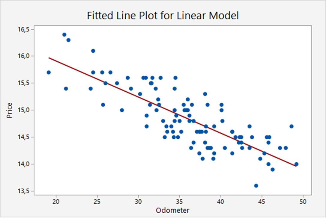
This scatter plot depicts the trade-in values for 100 basic models of a certain type of car, only based on the odometer readings, see Keller Example 16.2. There are 2 variables: Price and Odometer, so it is a univariate model. The blue dots represent the data (Price, Odometer) of each particular car. The red line is the so-called regression line. The regression line in this example is:

Price $=17248-0.066861$ Odometer

Least squares method

A scatter plot indicates the strength and direction of a linear relationship. Both can be more easily judged by drawing a straight line through the data. We need an objective method of producing such a straight line. Such a method has been developed; it is called the least squares method.

If we assume there is a linear relationship between two random variables $X$ and $Y$ we try to determine a linear function:

$\hat{y}=b_0+b_1x$ ( $b_0$ : the $y$ -intercept, $b_1$ : the slope of the line)

If $(x_i,y_i )$ represent the sample observations, then we want to draw the line such that the sum of the squared deviations (residuals) between the obervations and the corresponding points on the line is minimized, thus determine $b_0$ and $b_1$ such that $\sum_{}{}(y_i -\hat{y_i})^2$ is minimal.

The regression line

We solve the optimization problem by partial differentiation to $b_0$ and $b_1$ of the following function:

$\displaystyle{\sum_{}{}(y_i -\hat{y_i}})^2=\sum_{}{}(y_i-b_0-b_1x_i})^2}$

After some algebra we get:

$\displaystyle{b_1=\frac{s_{xy}}{{s_x}^2}}}$ and

$\displaystyle{b_0=\overline{y}-b_1\overline{x}}$