Sampling

Sampling distributions

(Keller 9)

A sample of size $n$ is just one of many possible samples of size $n$ . If $N$ is the population size and $n$ the sample size ( $n$ ≪ $N$ ) then the number of possible different samples equals $\displaystyle{\large{\binom{N}{n}}}$
This number of samples is usually very large. For example, from a population of 1000 objects the number of different samples of size 25 equals $\binom{100}{25}=2.4\cdot{10^{23}}$ .
Most samples have (different) random statistics, e.g. $\overline{x}$ or $s$ . These sample statistics have a probability distribution, the so-called sampling distribution.

Some mathematics

$\overline{X}$ and $s^2$ are sample statistics. Let us derive the distribution function of $\overline{X}$ . We know that $E(X)=\mu_{X}$ and $V(X)={\sigma_X^2}}$ . Then:

$\displaystyle{\mu_{\overline{X}}=E(\overline{X})=E(\frac{\sum{}{}X}{n})=\frac{\sum{}{}{E(X)}}{n}=\frac{nE(X}{n}=\frac{n\mu_{X}}{n}=\mu_X}$

$\displaystyle{{\sigma_{\overline{X}}^2=V(\overline{X})=V(\frac{\sum{}{}X}{n})=V(\frac{1}{n}\sum{}{}X)=}$

$\displaystyle{=\frac{1}{n^2}V(\sum{}{}X)=\frac{1}{n^2}\sum{}{}V(X)=\frac{1}{n^2}nV(X)=\frac{V(X)}{n}={\sigma_{{X}}^2}/n}$

So, for the random variable $\overline{X}$ it holds: $\mu_{\overline{X}}=\mu_X$ and $\displaystyle{\sigma_{\overline{X}}=\sigma_{X}/\sqrt{n}}$

Earlier we defined for any random variable $X$ :

$\displaystyle{Z=\frac{X-\mu_X}{\sigma_X}}$

and thus for the random variable $\overline{X}$ we get:

$\displaystyle{Z=\frac{\overline{X}-\mu_\overline{X}}{\sigma_\overline{X}}}=\frac{\overline{X}-\mu_X}{\sigma_{X}/\sqrt{n}}}$

Central Limit Theorem

(Keller 7, 8, 9)

The theorem states that he sampling distribution of the means of random samples drawn from any population is approximately normal for a sufficiently large sample size $n$ . The larger the sample size, the more closely the sampling distribution of $\overline{X}$ will resemble a normal distribution.

We will not prove the Central Limit Theorem here, that will be beyond the scope of this crash course. However, we try to make this theorem plausible by verifying it in a number of examples.

If the distribution of the population is normal, then $\overline{X}$ is normally distributed for all sample sizes $n$ . If the population is non-normal, then $\overline{X}$ is approximately normal only for larger values of $n$ . In most practical situations, a sample size of $n=30$ may be sufficiently large to allow us to use the normal distribution as an approximation for the sampling distribution of $\overline{X}$ .

Verify Central Limit Theorem (may be skipped)

(Keller 9)

The following is a program in pseudo code.

Take a first sample of size $n=30$ of a uniform distribution and compute its sample mean ${\overline{X}_1$ ;
Repeat this $k=5000$ times and thus get $5000$ sample means $\overline{X}_1\cdots\overline{X}_{5000}$ . Also these means are random variables;
According to the Central Limit Theorem these $5000$ random means should be (approximately) normally distributed;
Verify this graphically by drawing a histogram;
Verify this by applying a normality test (e.g. Anderson-Darling);
Repeat 1-5 for $n=1, 10, 30, 100$ and notice the differences.

The actual program is executed by the programming language R but any programming language will so. Thc code of the R program is as follows:

# Suppose x has a uniform distribution
# n is the sample size, preferably n = 30
n <- 30
# k is the number of such sample means, sufficiently large, e.g. k = 5000
k <- 5000
# According to the Central Limit Theorem
# the k sample means should approximate a normal distribution
z <- numeric(k) # z is a vector with k elements and will contain all k sample means
for (j in 1:k) (z[j] <- mean(runif(n))) # compute the mean of each uniform sample
# show the histogram of these means
hist(z)
# and find out whether the distribution of means is normal
# which is approximately true for n ≥ 30
ad.test(z) # Anderson-Darling test

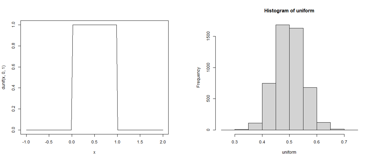
The result is as follows.

The left graph represents a uniform distribution on $[0,1]$ ; the right graph depicts a histogram of $5000$ sample means which is rather good approximation of a normal distribution.

Using the standard normal distribution

(Keller 9)

Suppose the population random variable $X$ is normally distributed with $\mu=32.2$ and $\sigma=0.3$ .

We take a sample of size $4$ drawn from the population. The sample mean is denoted by $\overling{X}$ . We want to compute $P(\overline{X}>32)$ .

We know:

$X$ is normally distributed, therefore so will be $\overline{X}$ .

$\displaystyle{\mu_{\overline{X}}=\mu_X=32.2}$ and $\displaystyle{\sigma_{\overline{X}}=\frac{\sigma_X}{\sqrt{4}}=\frac{0.3}{2}=0.15}$

$\displaystyle{P({\overline_{X}}>32)=P(Z>\frac{32-\mu_\overline{X}}{\sigma_\overline{X}}})$

$\displaystyle{=P(Z>\frac{32-32.2}{0.15})=P(Z>-1.333)=0.9082}$

The answer can be found in Table 3 of Appendix B9 of Keller.

The difference of two means

(Keller 9)

Consider the sampling distribution of the difference ${\overline{X}}_1-{\overline{X}}_2$ of two sample means.

If the random samples are drawn from each of two independent normally distributed populations, then ${\overline{X}}_1-{\overline{X}}_2$ will be normally distributed as well with:

$\displaystyle{\mu_{\overline{X}_1}-\mu_\overline{X}_2}=\mu_1-\mu_2}$

$\displaystyle{\sigma_{\overline{X}_1}-\sigma_\overline{X}_2}=}$

$\displaystyle{=\sqrt{{{\sigma_1}^2}/{n_1}+{{\sigma_2}^2}/{n_2}}}}$

If two populations are not both normally distributed, and the sample sizes are large enough ( $n>30$ ), then in most cases the distribution of ${\overline{X}}_1-{\overline{X}}_2$ is approximately normal (see the Central Limit Theorem).

Normal approximation to Binomial

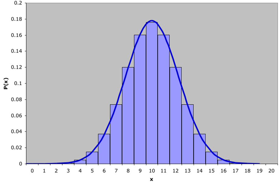
There are circumstances that a Binomial distribution may be approximated by a normal distribution. Let us look at the following example: a binomial distribution with $n=20$ and $p=0.5$ (so $\mu=np=10$ and $\sigma^2=np(1-p)=2.24$ ) superimposed by a normal distribution $N(10,2,24$ ).
The graph shows $P(0), P(1), \cdots, P(19), P(20)$ and the graph of a $N(10, 2.24)$ distribution.

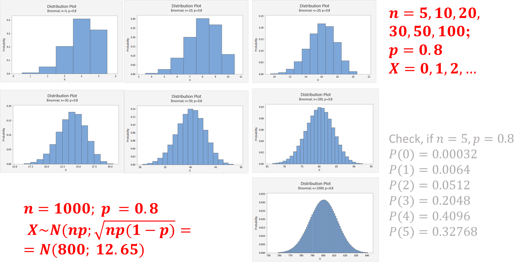
The normal approximation to binomial works best when the number of experiments $n$ is large and the probability of succes $p$ is close to $0.5$ .

For the approximation to provide acceptable results two conditions should be met:

$np\geq5$ and $n(1-p)\geq5$

Example
The following graph shows the approximations witp $p=0.8$ and various values of $n$ .

Example
How accurate is the approximation?
For a binomial distribution ( $n=20, p=0.5)$ we find (using Excel):
$P(X\leq13)=0.942341$ .
For a normal distribution ( $\mu=10, \sigma=2.24$ ) we find:
$P(X\leq13)=P(X\leq13.5)=0.940915$ (continuity correction), which is pretty close to the exact value.

Distribution of a sample proportion

The estimator of a population proportion of successes is the sample proportion. That is, we count the number of successes in a sample of size $n$ and compute:

$\displaystyle{\hat{p}=\frac{X}{n}}$

$X$ is the number of successes, $n$ is the sample size. Note that the random variable $X$ has a binomial distribution.
Using the laws of expected value and variance, we can determine the mean, variance and standard deviation. Sample proportions can be standardized to a standard normal distribution using the formula:

$\displaystyle{Z=\frac{X-\mu}{\sigma}$ and thus $\displaystyle{Z=\frac{\hat{p}-p}{\sqrt{p(1-p/n}}}}$

Note.
Binomial disribution: $X=p, E(X)=np, V(X)=np(1-p)$

$\displaystyle{E(\hat{p})=E(\frac{X}{n})=\frac{1}{n}E(X)=\frac{1}{n}\cdot{np}=p}$

$\displaystyle{V(\hat{p})=V(\frac{X}{n})=\frac{1}{n^2}V(X)=\frac{1}{n^2}np(1-p)=\frac{p(1-p)}{n}}$

and thus:

$\displaystyle{\sigma_{\hat{p}}=\sqrt{p(1-p)/n}$

Example
In the last election a state representative received $52$ % of the votes (so $p=0.52$ ; this can be considered as a population parameter!)
One year after the election the representative organized a survey that asked a random sample of $n=300$ people whether they would vote for him in the next election.
If we assume that his popularity has not changed what is the probability that more than half of the sample would vote for him?

The number of respondents who would vote for the representative is a binomial random variable with $n=300$ and $p=0.52$ and we want to determine the probability that the sample proportion is greater than $50$ %, That is, we want to compute $P(\hat{p}>0.50)$ .

From the foregoing we know that the sample proportion $\hat{p}$ is approximately normally distributed with mean $p=0.52$ and standard deviation $\sigma_{\hat{p}}=\sqrt{p(1-p)/n}=\sqrt{0.52(1-0.52)/300}=0.0288$

Thus we compute:

$\displaystyle{P(\hat{p}>0.50)=}$

$\displaystyle{=P(\frac{\hat{p}-p}{\sigma_{\hat{p}}}>\frac{0.50-0.52}{0.0288})=}$

$=P(Z>0.69)=0.7549$

If we assume that the level of support remains at $52$ % the probability that more than half the sample of $300$ people would vote for the representative is $75,49$ %.

Sampling

Sampling

Sampling distributions

Some mathematics

Central Limit Theorem

Verify Central Limit Theorem (may be skipped)

Using the standard normal distribution

The difference of two means

Normal approximation to Binomial

Distribution of a sample proportion

Contact

Tutor Math, Statistics or GMAT?

Language preference