Simple linear regression models
In the introduction to regression we discussed the (univariate) linear model:

where  and
and  are unknown population parameters which have to be estimated using some statistics. If
  and
and  are the estimates of
  and , respectively, then the regression line (the ‘best’ approximation) is:

What is defined as the ‘best’ and how and are computed and for other details we refer to the introduction to regression.
Example
This example will use Excel.
A used-car dealer randomly selected 100 three-year old Toyota Camrys that were sold at auctions during the past month in order to determine the regression line price vs. odometer readings. The scatter plot (see the graph below) suggests a linear relation. The dealer recorded the price (in 1,000s) and the number of miles (in thousands) on the odometer.
Excel provides the following output.
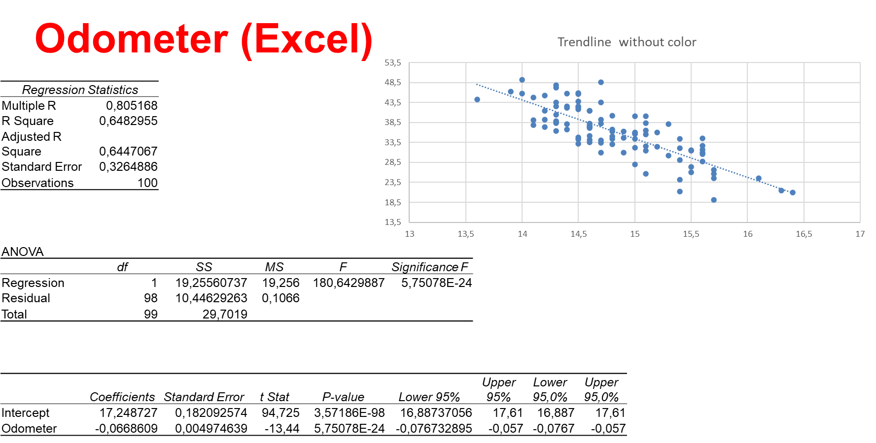
Important output data are the coefficient of determination  in the Regression Statistics table, the
  value and its
  value in the ANOVA table, and the values of the coefficients and their values in the coefficients table. We will discuss them later.
The coefficients of the regression line are used in the following formula.

Requirements
For the regression methods to be valid the following four conditions for the error variable  must be met:
- The probability distribution of is normal;
- The mean of the distribution is
 ; that is
  ;
; - The standard deviation
 is a constant regardless of the value of
  ;
; - The value of associated with any particular value of is independent of associated with any other value of {y} (important only for time series).
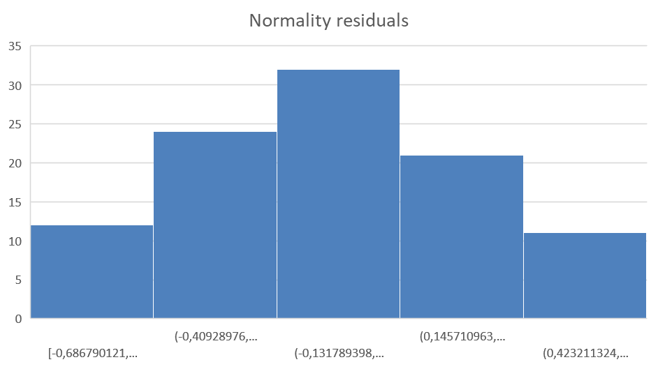
In the graph below the frequency diagram of the residuals is depicted. The residuals seem to be normally distributed with zero mean which meets the first requirement. A more quantitative method is the Anderson-Darling test.
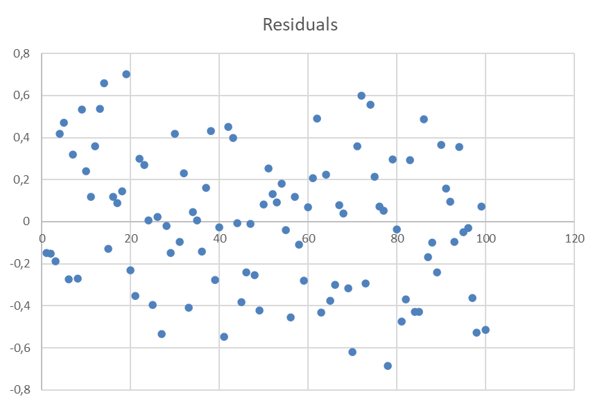
The diagram below shows that the variance of the residuals seems independent of the values.
Testing the slope
If no relationship exists between the two variables, we would expect the regression line to be horizontal, that is, to have a slope equal to zero. We want to find out if there is a linear relationship, i.e. we want to find out if the slope  . Then our research hypothesis is:

and the null hypothesis becomes:

We can implement the following test statistic to try our hypotheses:

Usually  is taken 0, because usually
  .
.

If the error variable  is normally distributed, the test statistic has a Student’s
  distribution with
  degrees of freedom. The rejection region depends on whether or not we are doing a one or two tail test (two-tail test is most typical).
In the Odometer example we get:

and thus the test statistic is:

Note.  is the standard error and can be found in the coefficient table.
The rejection region (two-sided) is:
 or
or 
or
 or
or 
The test statistic is in the rejection region and thus we reject .
Testing the coefficient of correlation
Also in the Odometer example we investigate the following hypotheses:

First we computer the sample coefficient of correlation:

The test statistic is:

which certainly falls into the rejection region:
 or
or
and thus there is overwhelming evidence to reject  .
.
Coefficient of determination
Thus far we tested whether a linear relationship exists; it is also useful to measure to what extent the model fits the data. This is done by calculating the coefficient of determination .

Note. If  (i.e. all points lie on the regression line) then
  and the model fits the data perfectly.
or

In the Odometer example we found  . This means that
  % of the variation in the auction selling prices is explained by the variation in the odometer readings
  . The remaining
  % is unexplained, i.e. due to error.
Unlike the value of a test statistic, the coefficient of determination does not have a critical value that enables us to draw conclusions. In general, the higher the value of , the better the model fits the data: (perfect fit);  (no fit).
If we have the regression equation:

then we can use it for any  to estimate intervals for
There are two types of intervals for  :
:
Prediction interval:

Confidence interval:

What is the difference between these two intervals? The prediction interval concerns an individual trade-in price while the second interval can be compared with the expected value: the mean trade-in price.
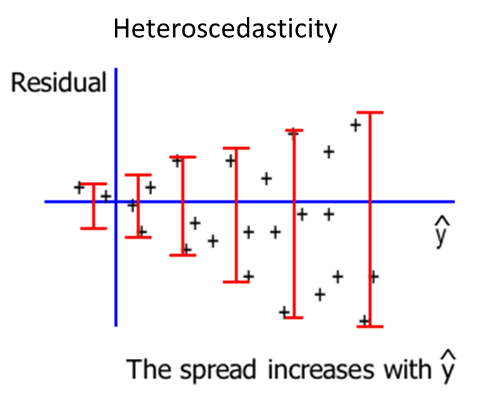
Homo- and heteroscedasticity
When the requirement of a constant variance is violated, we have a condition of heteroscedasticity. If it is not violated then we have a condition of homoscedasticity. We can diagnose heteroscedasticity by plotting the residual against the predicted .
In the Odometer example the graph shows the plot of the residuals against the predicted value of .
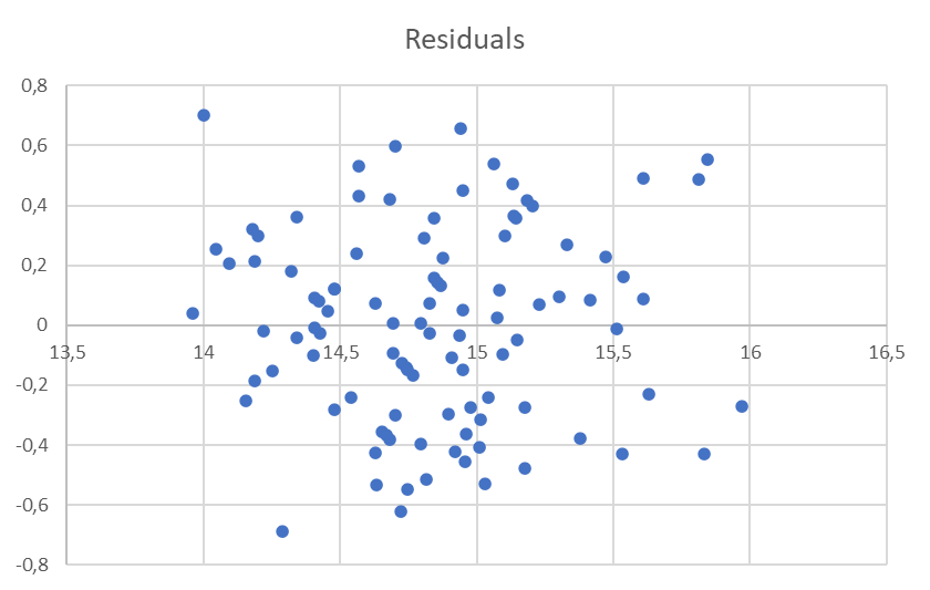
There doesn’t appear to be a change in the spread of the plotted points, therefore homoscedastic. (Question: Which flights have greater variability of air time: Amsterdam-Singapore or Amsterdam-Madrid?)