Multiple regression

In many applications there are more independent linear variables $x_i$ .

Then the model equation is:

$y=\beta_0+\beta_1x_1+\beta_2x_2\cdots+\beta_kx_k+\varepsilon$

and the regression equation is, based on the observation data:

$\hat{y}=b_0+b_1x_1+b_2x_2\cdots+b_kx_k$

The regression coefficients $b_i;(i=0,1,2,\cdots,k)$ are computed by software.

Example
Let us look at the following example. You want to determine the rate of a room in a new hotel. How would you do that? Relevant parameters are: city, distance of hotel to center or highway, luxury, how many hotels nearby (competitors), how many rooms, rates in other hotels etc.
Build a multiple regression model based on these independent variables $(x_i)$ and the dependent variable.

See also General Social Survey (variables that affect income). See Keller p. 686.

Requirements are the same as in univariate models. The coefficient of determination $R^2$ has the same function. If $R^2$ is close to $1$ then the model fits the data very well. If $R^2$ is close to $0$ then the model fits the data very poorly. The ANOVA technique tests the validity (the linearity) of the model. The hypotheses for this part are:

$\displaystyle{H_0: \beta_0=\beta_1\cdots=\beta_k=0}$ ;

$\displaystyle{H_1:$ at least one $\beta_i\neq=0}$ .

If the test statistic $F>F_{k-1,n-k-1;\alpha$ (the rejection region), then reject $H_0$ and at least one $\beta_i\neq0$ ,meaning that the model is valid (there is a linear relation with at least one $x_i$ ).

Testing the individual coefficients

For each individual independent variable, we can test whether there is enough evidence of a linear relationship between the output $y$ and a specific input variable $x_i$ ..

The hypotheses are:

$H_0: \beta_i=0; H_1: \beta_i\neq0; (i=1, 2, \cdots, k)$

The test statistic is:

$\displaystyle{t=\frac{b_i-\beta_i}{s_{b_i}}=\frac{b_i}{s_{b_i}}}$

If $\displaystyle{t<-t_{n-k-1;\alpha/2}}$ or $t>t_{n-k-1; \alpha∕2}}$ then reject $H_0$ .

Note. Reject if $p<\alpha/2$ or $2p<\alpha$ .

Multicollinearity

Multiple regression models have a problem that simple regression models do not have, namely multicollinearity. It happens when one or more independent variables are (highly) correlated.

The adverse effect of multicollinearity is that the estimated regression coefficients of the independent variables that are correlated, tend to have large sampling errors.

Example
A linear model expresses the relation of someone's lottery expenses (dependent variable $y$ ) and a number of characteristics such as Education, Age, Children and Income (independent variables). The table below shows that the correlations between the variables (Income, Education) and (Age, Education) are significant, leading to multicollinearity.

Nonlinear models

Regression analysis is used for linear models using interval data, but regression analysis can also be used for: non-linear (e.g. polynomial) models, and models that include nominal (also called dummy) independent variables,

Previously we looked at this multiple regression model:

$y=\beta_0+\beta_1x_1+\beta_2x_2+\cdots+\beta_kx_k+\varepsilon$

The independent variables $x_i$ may be functions of a smaller number of so-called predictor variables. Polynomial models fall into this category. If there is one predictor value $x$ we have:

$y=\beta_0+\beta_1x+\beta_2x^2+\cdots+\beta_px^p+\varepsilon$

We can rewrite this polynomial model:

$y=\beta_0+\beta_1x_1+\beta_2x_2+\cdots+\beta_px_p+\varepsilon$

Two predictor variables (linear and quadratic)

Suppose we assume that there are two predictor variables $\displaystyle{x_1}$ and $\displaystyle{x_2}$ which linearly influence the dependent variable $y$ . Then we can distinguish between two types of models.

One is a first order model without interaction between $\displaystyle{x_1}$ and $\displaystyle{x_2}$ .

$\displaystyle{y=\beta_0+\beta_1x_1+\beta_2x_2+\varepsilon}$

The second model is with interaction between $x_1$ and $x_2$ .

$\displaystyle{y=\beta_0+\beta_1x_1+\beta_2x_2+\beta_3x_1x_2+\varepsilon}$

Usually, we cannot give a meaning to the interaction term.

If we assume a quadratic relationship between $y$ and each of $x_1$ and $x_2$ , and that these predictor variables interact in their effect on $y$ , we can use this second order model (with two independent variables) with interaction:

$y=\beta_0+\beta_1x_1+\beta_2x_2+\beta_3x_1^2+\beta_4x_2^2+\beta_5x_1x_2+\varepsilon$

Example
We want to build a regression model for a fast food restaurant and know that its primary market is middle income adults and their children, particularly those between the ages of 5 and 12. In this case the dependent varuable is the restaurant revenue and the predictor variables are family income and the age of children. A question is whether the relationship is first order, quadratic, with or without interaction. The significance level is $5$ %.

An indication for a quadratic relationship can be found in the scatterplots. You can take the original data collected (revenues, household income, and age) and plot $y$ vs. $x_1$ and $y$ vs. $x_2$ to get a feel for the data, with the following results.

Based on the graphs we prefer a second order model (with interaction):

$y=\beta_0+\beta_1x_1+\beta_2x_2+\beta_3x_1^2+\beta_4x_2^2+\beta_5x_1x_2+\varepsilon$

although we cannot give a meaning to the interaction term.

The result is given in the following Excel table.

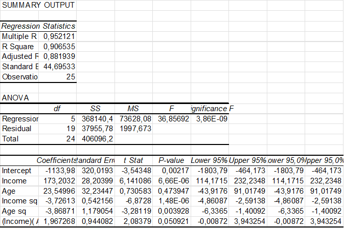
The coefficient of determination $R^2=90.65%$ is rather high indicating that the model fits the data very well. The $p$ value of $F$ is very small $<<0.0001$ , so the model is valid (at least one coeffincient is unequal zero). The coefficients Income, Income sq, Age sq have very small $p$ values and may be assumed to be linearly related. Age and IncomeAge don’t seem to be linearly related, because their $2p$ are greater than 0.05. Note. Reject $H_0:$ variable $= 0$ if $2p >\alpha$ (two-sided test).

So, we may conclude that the model fits the data very well, is valid and the coefficients of the variables Age and IncomeAge might be assumed to be 0 amd thus these variables do not seem to be releated to the revenu.

Nominal variables

Thus far in our regression analysis, we have only considered interval variables. Often however, we need to consider nominal data in our analysis. For example, our earlier example regarding the market for used cars focused only on the interval variable Odometer. But the nominal variable color may be an important factor as well? How can we model this new nominal variable?

An indicator variable (also called a dummy variable) is a variable that can assume either one of only two values (usually 0 and 1). A value of 1 usually indicates the existence of a certain condition, while a value of 0 usually indicates that the condition does not hold.

Car color	$I_1$	$I_2$
white	1	0
silver	0	1
other	0	0
two-tone	1	1

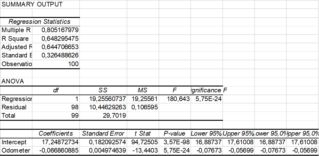
Let us consider the difference between the regression models without and with color. See the following Excel output.

Without color

With color

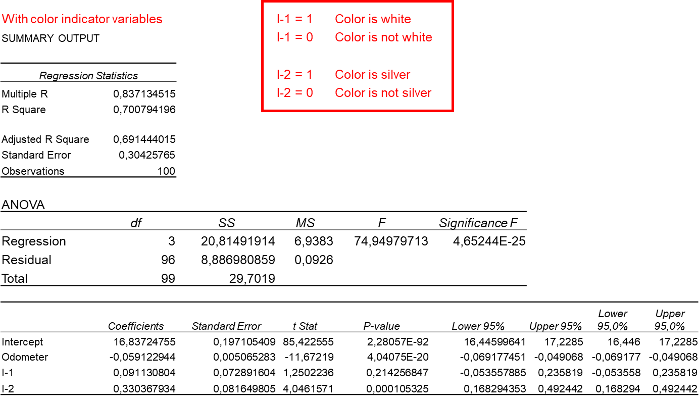
In the case 'without color' the coefficient of determination $R^2$ is less than in the case 'with color'. The latter model fits the data a bit better. Another conclusion is that a white car sells for 91.10 dollars more than other colors and a silver car sells for 330.40 dollars more than other colors (*). However, for the $p$ value of $I1$ we have $2p>0.05$ so it seems that the color white does not seem to be related to the price.