Hypothesis testing (one population)

There are two hypotheses, the null hypothesis $H_0$ and the alternative or research hypothesis $H_1$ or $H_a$ . The procedure begins with the assumption that the null hypothesis is true and the goal is to determine whether there is enough evidence to support the alternative hypothesis. There are two possible decisions:

There is enough evidence to support the alternative hypothesis and to reject the null hypothesis; or
There is not enough evidence to support the alternative hypothesis and to not reject the null hypothesis.

The procedure

Collect sampling data (e.g. $x_1, \cdots, x_n}$ );
Calculate some statistic, e.g. $\overline{X}$ if the hypothesis is about the population mean $\mu$ ;
See whether the statistic is extreme or is seen as “bad luck”, given $H_0$ ( $H_0$ is assumed to be correct);
If extreme, reject $H_0$ ;
If not extreme, do not reject $H_0$ .

So, reject $H_0$ when the result is extreme, but what is extreme? We consider extreme: (very) unlikely under $H_0$ . However how unlikely is unlikely? This choice has to made by the statistician: the significance level $\alpha$ . This is usually set at $5$ % but also $1$ % or $10$ % are common.

Reject if the statistic is in the $\alpha$ tail of the distribution under $H_0$ We can also say: if $H_0$ is correct, reject in $\alpha$ % of the cases.

Potential errors

There are two types of error.

Type I error
Reject $H_0$ while $H_0$ is correct.
Based on the data you find the result extreme and reject $H_0$ but after all $H_0$ appears to be correct.

Type II error
Do not reject $H_0$ while $H_0$ is not correct.
Based on the data you find the result “acceptable” and you do not reject $H_0$ but after all $H_0$ appears not to be correct.

Example

The Dutch coffee brewer Douwe Egberts sells packs of coffee. It claims that the mean weight of the packs is 250 grams or more. The population standard deviation is known: $\sigma=3$ grams. To verify this claim we take a sample of $9$ packs.
What would we decide if you find $\overline{X}=247$ grams? Reject or not reject $H_0$ ? And why?
This is one-sided problem.

We have the following data:
$n=9$ packs
$\mu=$ 250 grams (the claim)
$\sigma=3$ grams
$\overline{X}=247$ grams
$H_0: \mu=250$ grams; $H_1: \mu<250$ grams

We compute the probability of 'bad luck', i.e. we assume $H_0$ is true and yet we find $\overline{}=247$ :

$\displaystyle{P(\overline{X}<247 | \mu=250)=P(Z<\frac{247-250}{3/\sqrt{9}})=}$

$\displaystyle{=P(Z<-3.0)=0.0013}$

This means that if such a sample would be taken every day during about 3 years, only once the result would be $247$ grams or less. Would we decide this as 'very unlikely under $H_0$ '? What would we decide: reject or not reject $H_0$ ?

If we would decide the probability $P(Z<-3.0)=0.0013$ is too small to not reject the null hypothesis, what probability would be acceptable: $0.005$ , $0.01$ , $0.05$ ? This choice is determined by the significance level $\alpha$ . A common choice is $\alpha=0.05$ . In this case we find the sample mean very extreme under $H_0$ and would reject the null hypothesis.

Example

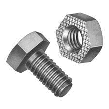
Now we consider a pair of nuts and bolts. The manufacturer claims that the diameter of the bolts is 1 cm, not larger or smaller. The population standard deviation is $\sigma=0.03$ cm. To verify this claim we take a sample of $9$ bolts.

What would we decide if we find $\overline{X}=1.03$ cm. Reject or not reject $H_0$ ? And why? This is two-sided problem.

We have the following data:

$n=9$ bolts
$\mu=1$ cm
$\sigma=0.03$ cm
$\overline{X}=1.03$ cm
$H_0: \mu=1$ cm; $H_1: \mu\neq1$ cm

We compute the probability of 'bad luck', i.e. $H_0$ is true and yet we find $\overline{}=1.03$ :

$\displaystyle{P(\overline{X}>1.03 | \mu=1)=P(Z>\frac{1.03-1.0}{3/\sqrt{9}})=}$

$\displaystyle{=P(Z>3.0)=0.0013}$

Again we would reject the null hypothesis.

Suppose that the sample mean would be $\overline{X}=0.97$ Then we would find:

$P(Z<-3.0)=0.0013$

and we would again reject the null hypothesis.
If the significance level $\alpha=0.05$ , in the one-sided coffee case we would reject the null hypothesis because $p<\alpha$ , namely ( $0.003<0.05$ ).

In the nuts and bolts case we would reject the null hypothesis if $2p<\alpha$ ( $2\cdot{0.003}<0.05$ ) (both too large or too small is not acceptable).

Rejection region

The rejection region is a range of values such that if the test statistic falls into that range, we decide to reject the null hypothesis in favor of the alternative hypothesis. The rejection region is usually used when the test is carried out manually.

One-sided or two-sided

Depending on the alternative hypothesis the test is either one-sided or two-sided.

If $H_0: \mu=A, H_1: \mu>A$ or $H_1: \mu<A$ the hypothesis test is called one-sided.
If $H_0: \mu=A, H_1: \mu\neq{A}$ the hypothesis test is called two-sided.

Strategies to perform the test

Strategy 1: Use the rejection region if the test is carried out manually.

Choose the significance level $\alpha$ ;
Calculate the test statistic, e.g. based on $\overline{X}$ ;
Calculate the rejection region;
Reject $H_0$ if the test statistic is in the rejection region.

Strategy 2: use the $p$ -value if the test is carried out by computer.

Choose the significance level $\alpha$ ;
Calculate the test statistic, e.g. based on $\overline{X}$ ;
Calculate its probability under $H_0$ which results in a $p$ -value;
Reject $H_0$ if $p<\alpha$ (one-sided) or $2p<\alpha$ (two-sided).

The Z test

If we want to perform a one-sided hypothesis test with:

$\displaystyle{H_0: \mu=\mu_0, H_1: \mu>\mu_0}$

and $\sigma$ is known, then use the data to compute $\overline{X}$ and compute the test statistic:

$Z=\displaystyle{\frac{\overline{X}-\mu_0}{\sigma/\sqrt{n}}$ .

Define $Z_\alpha$ from $P(Z>Z_\alpha)=\alpha$ .

The rejection region is $Z>Z_\alpha$ and reject $H_0$ if $Z$ falls into the rejection region. Often used values are: $Z_{0.05}=1.645$ (one-sided) and $Z_{0.025}=1.96$ (two-sided). See Keller, table B.3.
If we want to perform a one-sided hypothesis test with:

$\displaystyle{H_0: \mu=\mu_0, H_1: \mu<\mu_0}$

and $\sigma$ is known, then use the data to compute $\overline{X}$ and compute the test statistic:

$Z=\displaystyle{\frac{\overline{X}-\mu_0}{\sigma/\sqrt{n}}$ .

Define $Z_\alpha$ from $P(Z<-Z_\alpha)=\alpha$ .
The rejection region is $Z<-Z_\alpha$ and reject $H_0$ if $Z$ falls into the rejection region.
If we want to perform a two-sided hypothesis test with:

$\displaystyle{H_0: \mu=\mu_0, H_1: \mu\neq{\mu_0}}$

and $\sigma$ is known, then use the data to compute $\overline{X}$ and compute the test statistic:

$Z=\displaystyle{\frac{\overline{X}-\mu_0}{\sigma/\sqrt{n}}$ .

Define $Z_\alpha/2$ from $P(Z<-Z_\alpha)=\alpha/2$ .
The rejection region is $Z<-Z_\alpha/2$ or $Z>Z_\alpha/2$ and reject $H_0$ if $Z$ falls into the rejection region.

We look at the rejection region vs. the $p$ -value and consider again the one-sided test of the previous coffee examples.

Strategy 1 (one-sided)

First we look at the case $\overline{X}=247$ .

$H_0: \mu=250; H_1: \mu<250; \sigma=3; n=9; \alpha=0.05; \overline{X}=247$

The test statistic is:

$\displaystyle{Z={\frac{247-250}{3/\sqrt{9}}=-3}$

$\displaystyle{Z_{0.05}=1.645}$

The rejection region is:

$\displaystyle{Z<-1.645}$ .

The test statistic is in the rejection region.

Conclusion: reject $H_0$ .

Now the case $\overline{X}=249$

$H_0: \mu=250; H_1: \mu<250; \sigma=3; n=9; \alpha=0.05; \overline{X}=249$

The test statistic is:

$\displaystyle{Z={\frac{249-250}{3/\sqrt{9}}=-1}$

$\displaystyle{Z_{0.05}=1.645}$

The rejection region is:

$\displaystyle{Z<-1.645}$ .

The test statistic is not in the rejection region.

Conclusion: do not reject $H_0$ .

Strategy 2 (one-sided)

First we look at the case $\overline{X}=247$ .

$H_0: \mu=250; H_1: \mu<250; \sigma=3; n=9; \alpha=0.05; \overline{X}=247$

The test statistic is:

$\displaystyle{Z={\frac{247-250}{3/\sqrt{9}}=-3}$

We find:

$\displaystyle{p=P(Z<-3)=0.0013}$

Since:

$p<\alpha$ $(0.0013<0.05)}$

we reject the null hypothesis $H_0$ .

Now we consider the case $\overline{X}=249$ .

$H_0: \mu=250; H_1: \mu<250; \sigma=3; n=9; \alpha=0.05; \overline{X}=249$

The test statistic is:

$\displaystyle{Z={\frac{247-250}{3/\sqrt{9}}=-1}$

We find:

$\displaystyle{p=P(Z<-1)=0.1587}$

Since:

$p>\alpha$ $(0.1587>0.05)}$

we do not reject the null hypothesis $H_0$ .

Now we look at the two-sided test of the nuts and bolts example.

Strategy 1 (two-sided)

$H_0: \mu=1; H_1: \mu\neq{1}; \sigma=0.03; n=9; \alpha=0.05; \overline{X}=1.03$

The test statistic is:

$\displaystyle{Z={\frac{1.03-1.00}{0.03/\sqrt{9}}=3}$

$Z_{0.025}=1.96$

The rejection region is:

$\displaystyle{Z<-1.96}$ or $Z>1.96$ .

The test statistic is in the rejection region. So, we reject the null hypothesis $H_0$

Strategy 2 (two-sided)

Now we look at the case when $\overline{X}=1.01$ .

$H_0: \mu=1; H_1: \mu\neq{1}; \sigma=0.03; n=9; \alpha=0.05; \overline{X}=1.01$

The significance level is $\alpha=0.05$ , so $\alpha/2=0.025$

The test statistic is:

$\displaystyle{Z={\frac{1.01-1.00}{0.03/\sqrt{9}}=1}$

We find $P(Z>1)=0.1587$ .
So, the $p$ -value equals $0.1587$ . Since $p>\alpha/2$ $(0.1587>0.025)$ we do not reject the null hypothesis $H_0$ .

What if the population is not normal?

Suppose that the requirement $X$ is normally distributed is violated? In cases where $n$ is large (about $30$ or more) this is not really a problem because of the Central Limit Theorem. If $n$ is not large enough we can't rely on the $Z$ -test. Then we need to use so-called nonparametric tests, e.g. the Wilcoxon signed rank test.

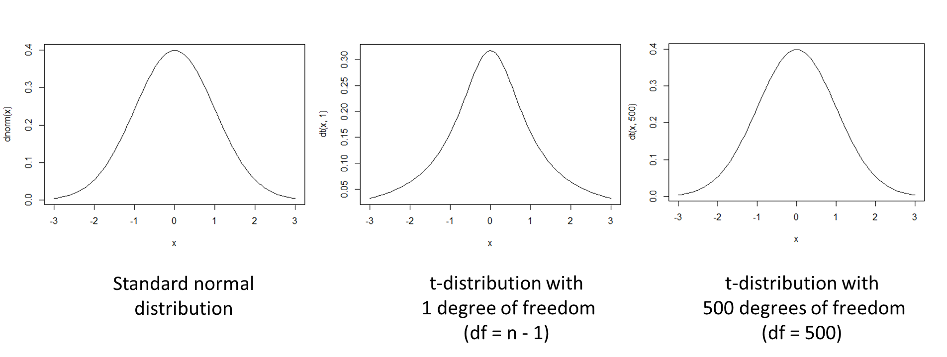
Hypothesis testing, unknown population variance

Thus far the population standard deviation $\sigma$ is assumed to be known and then we could use the test statistic:

$\displaystyle{Z=\frac{\overline{X}-\mu}{\sigma/\sqrt{n}}}$

If $\sigma$ is unknown which is almost always the case, we use $\sigma$ ’s point estimator $s$ instead and get the test statistic:

$\displaystyle{t_{n-1}=\frac{\overline{X}-\mu}{s/\sqrt{n}}}$

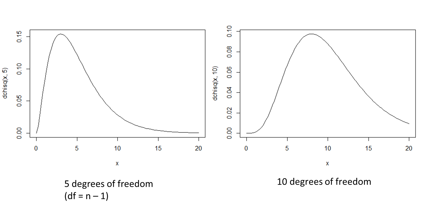
which has a so-called Student's $t$ -distribution. $n-1$ is called degrees of freedom, written as $\nu$ or $df$ . All distributions $t_{\nu}$ have a symmetrical graph around $t=0$ and approximate the standard normal distribution $N(0,1)$ for larger $n$ :

$\displaystyle{\lim_{n \to \infty} {t_n}}=Z}$

The t test

If we want to perform a one-sided hypothesis test with:

$H_0: \mu=\mu_0, H_1: \mu>\mu_0$

then use the data to compute $\overline{X}$ and $s$ and the test statistic:

$\displaystyle{t=\frac{\overline{X}-\mu}{s∕\sqrt{n}}}$

Next, find $\displaystyle{t_{\nu;\alpha}}$ and the rejection region is

$\displaystyle{t>t_{\nu;\alpha}}$

Reject $H_0$ if $t$ falls into the rejection region

Use a similar approach when $H_1:\mu<\mu_0$ and If the test is two-sided use $t_{\nu;\alpha/2}$

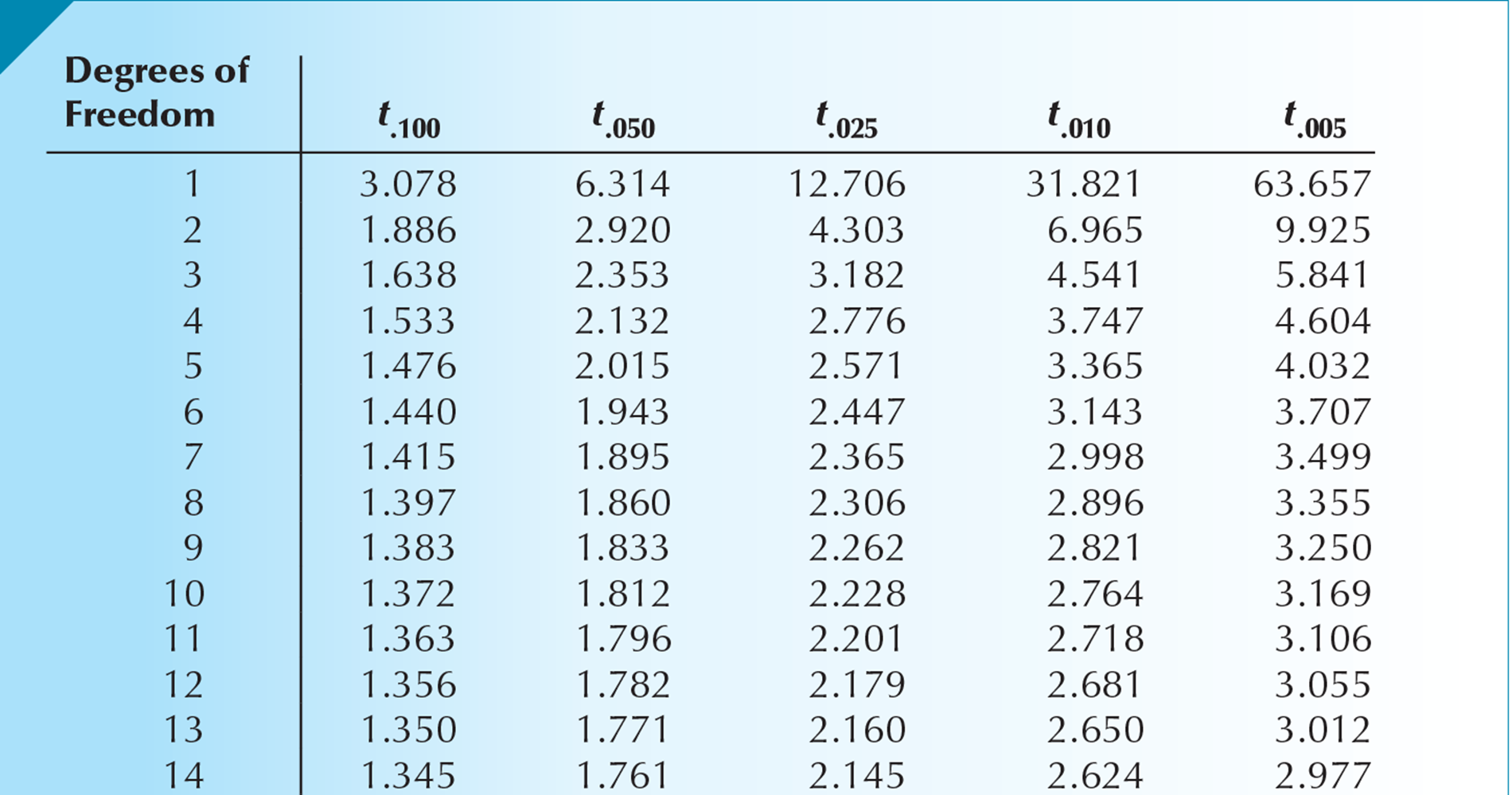
Example
If $n=11$ then $\nu=10$
$t_{10;0.05}=1.812$
$t_{10;0.025}=2.228$
See the table below.

Inference about the population variance

If we are interested in drawing inferences about a population’s variability, the parameter we need to investigate is the population variance. The sample variance $s^2$ is an unbiased, consistent and efficient point estimator of $\sigma^2$ . Moreover, the test statistic:

$\displaystyle{\chi^2=\frac{(n-1)s^2}{\sigma^2}}$

has a $\chi^2$ distribution with $\nu=n-1$ degrees of freedom.

Confidence interval of the variance

Combining the test statistic:

$\displaystyle{\chi^2=\frac{(n-1)s^2}{\sigma^2}}$

with the probability statement:

$\displaystyle{P({\chi^2}_{\nu; 1-\alpha/2}<\chi^2<{\chi^2}_{\nu; \alpha/2}=1-\alpha}$

yields the confidence interval estimator for $\sigma^2$ :

Lower confidence Limit $<\sigma^2<$ Upper confidence limit:

$\displaystyle{\frac{(n-1)s^2}{{\chi^2}_{\nu;\alpha/2}}<\sigma^2<\frac{(n-1)s^2}{{\chi^2}_{\nu;{1-\alpha/2}}}}$

Graphs of the Chi-squared distribution

What does the procedure look like in the one-sided (left and right) or two-sided case.

One-sided left
In this case we have:

$\displaystyle{H_0:\sigma^2=A; H_1:\sigma^2<A}$

and the significance level is $\alpha$ .

Compute the test statistic:

$\displaystyle{\chi^2=\frac{(n-1)s^2}{\sigma^2}}$

and find (use table 5, p. B-11):

$\displystyle{{\chi^2}_{\nu;1-\alpha}}$

The rejection region is

$\displaystyle{\chi^2<{\chi^2}_{\nu;1-\alpha}}$ .

And thus reject $H_0$ if:

$\displaystyle{\chi^2<{\chi^2}_{\nu;1-\alpha}}}$

One-sided right
The procedure is similar. In this case we have:

$\displaystyle{H_0:\sigma^2=A; H_1:\sigma^2>A}$

and the significance level is $\alpha$ .

Compute the test statistic:

$\displaystyle{\chi^2=\frac{(n-1)s^2}{\sigma^2}}$

and find (use table 5, p. B-11) $\displystyle{{\chi^2}_{\nu;\alpha}}$ . The rejection region is:

$\displaystyle{\chi^2>{\chi^2}_{\nu;\alpha}}$ .

And thus reject $H_0$ if

$\displaystyle{\chi^2>{\chi^2}_{\nu;\alpha}}}$

Two-sided
In this case we have:

$\displaystyle{H_0:\sigma^2=A; H_1:\sigma^2\neq{A}}$

and the significance level is $\alpha$ .

Compute the test statistic:

$\displaystyle{\chi^2=\frac{(n-1)s^2}{\sigma^2}}$

and find (use table 5, p. B-11) $\displystyle{{\chi^2}_{\nu;\alpha/2}}$ and $\displystyle{{\chi^2}_{\nu;1-\alpha/2}}$ .
The rejection region is:

$\displaystyle{\chi^2<{\chi^2}_{\nu;1-\alpha/2}}$ or $\displaystyle{\chi^2>{\chi^2}_{\nu;\alpha/2}}$

And thus reject $H_0$ if $\chi^2$ falls into the rejection region.

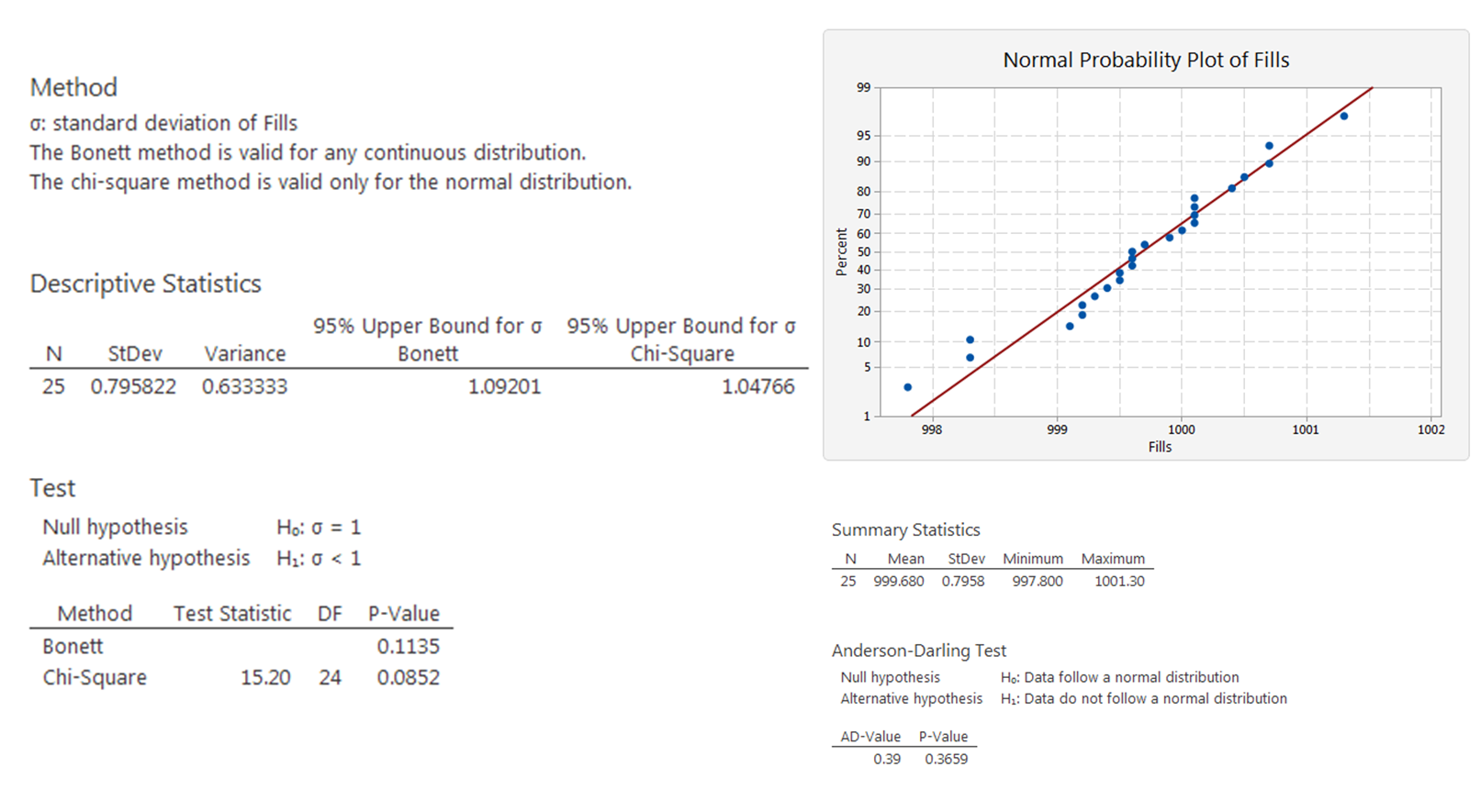
A container filling machine

Container-filling machines are used to package a variety of liquids, including milk, soft drinks, or paint. Ideally, the amount of liquid should vary only slightly, since large variations will cause some containers to be underfilled and some to be overfilled (resulting in a mess).

The president of a company that developed a new type of machine boasts that this machine can fill 1 liter (1,000 cubic centimeters) containers so consistently that the variance of the fills will be less than 1 cubic centimeter.

A sample of 25 fills of 1 liter was taken showing $s^2=0.6333$ .
The null and alternative hypotheses are:

$H_0: \sigma^2=1; H_1: \sigma^2<1; n=25; \alpha=0.05$

The test statistic is:

$\displaystyle{\chi^2=\frac{(n-1)s^2}{\sigma^2} =15.20$

The rejection region is:

$\displaystyle{\chi^2<{\chi^2}_{\nu;1-\alpha}}={\chi^2}_{24;0.95}}=13.85}$

The test statistic $\chi^2=15.20$ is not less than 13.85 and thus not in the rejection region, so we do not reject the null hypothesis in favor of the alternative hypothesis.

This example has been computed by Minitab Express with the following results. Just look at the $\chi^2$ data, because the Anderson-Darling test shows that the data are normally distributed. The computed $p=0.0852>0.05$ so we will not reject the null hypothesis.

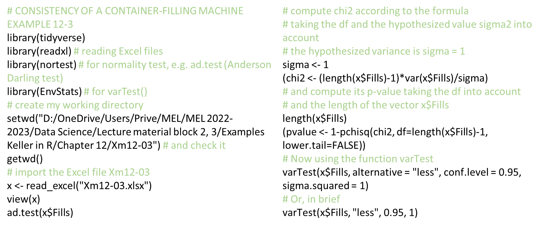
Also the programming language R can do the job. See the program below.

Test statistic for proportions

If $n$ is the sample size, $p$ is the assumed population proportion and $\displaystyle{\hat{p}=\frac{x}{n}}$ ( $x$ the number of successes in the sample) is the estimate of $p$ , then the test statistic for proportions is:

$Z=\displaystyle{\frac{\hat{p}-p}{\sqrt{p(1-p)/{n}}}$

which is approximately normal when $np$ and $n(1-p)$ are both greater than 5. (Note: the normal approximation of binomial distribution).

Compare this formula with:

$\displaystyle{Z=\frac{\overline{X}-\mu_{\overline{X}}}{\sigma_{\overline{X}}}=\frac{\overline{X}-\mu}{\sigma/\sqrt{n}}}$

To understand the test statistic for proportions, recall the following (binomial) formulas:

$E(X)=np$ ; $E(\hat{p})=p$

$V(X)=np(1-p)$ ; $V(\hat{p})=p(1-p)/n$

$\sigma_{\hat{p}}=\sqrt{p(1-p)/n}$

Example: An exit poll
An exit poll of $n=765$ voters showed that $407$ $(x)$ voted for the Republican candidate. Thus:

$\displaystyle{\hat{p}=\frac{x}{n}=0.532}$

Suppose $H_0: p=0.5$ , (Dems win); $H_1: p>0$ (Reps win).

The test statistic is:

$Z=\displaystyle{\frac{\hat{p}-p}{\sqrt{p(1-p)/{n}}}=\frac{0.532-0.5}{\sqrt{0.5(1-0.5)/765}}=1.77}$

If the signicance level is $\alpha=5$ % we know that the rejection region is $Z>Z_{0.05}=01.645$ . Because $Z$ is in the rejection region we reject the null hypothesis.

So, there is enough evidence at the 5% significance level that the Republican candidate will win.