Hypothesis testing (two or more populations)

Following we will look at comparing and testing two or more populations.

Comparing the means $\mu_1$ and $\mu_2$ ;
Comparing the variances ${\sigma_1^2$ and ${\sigma_2^2$ ;
Comparing the proportions $p_1$ and $p_2$ .

We also compare the means of three or more populations (ANOVA).

Previously we looked at techniques to estimate and test parameters of one population:

Population mean $\mu}$ ;
Population variance $\sigma^2}$ ;
Population proportion $p$ .

We will still consider these parameters when looking at two populations or more, however, our interest will now be:

The difference of two population means $\mu_1-\mu_2$ ;
The ratio of two population variances $\displaystyle{\frac{{\sigma_1}^2}{{\sigma_2}^2}}$ ;
The difference of two population proportions $p_1- p_2$ .

Comparing two population means

If we compare two population means, we use the statistic ${\overline{X}}_1- {\overline{X}}_2$

${\overline{X}}_1$ is an unbiased and consistent estimator of $\mu_1$ ;
${\overline{X}}_2$ is an unbiased and consistent estimator of $\mu_2$ ;
Then ${\overline{X}}_1- {\overline{X}}_2$ is an unbiased and consistent estimator of $\mu_1-\mu_2$ .

Note. Usually, the sample sizes $n_1$ and $n_2$ are not equal.

We consider two cases.

Independent populations. The data in one population are independent of the data in the other population;
Matched pairs. Observations in one sample are matched with observations in the second sample, so the samples are not independent.

Independent populations

The random variable ${\overline{X}_1}-{\overline{X}_2}$ is normally distributed if the original populations are normal or approximately normal if the populations are nonnormal and the sample sizes are large enough ( $n_1,n_2>30$ , Central Limit Theorem).

Earlier we derived:

$\displaystyle{E({\overline{X}}_1-{\overline{X}}_2)=\mu_1-\mu_2}$

$\displaystyle{V({\overline{X}}_1-{\overline{X}}_2)=\frac{\sigma_1^2}{n_1}+\frac{\sigma_2^2}{n_2}}$

So, the standard error is:

$\displaystyle{\sigma_{{\overline{X}}_1- {\overline{X}}_2}}=\sqrt{\frac{\sigma_1^2}{n_1}+\frac{\sigma_2^2}{n_2}}}$

If $\overline{X}_1-\overline{X}_2$ is (approximately) normally distributed and $\sigma_1^2-\sigma_2^2$ are known, then the test statistic is:

$\displaystyle{Z=\frac{(\overline{X}_1-\overline{X}_2)-(\mu_1-\mu_2)}{\sqrt{\frac{\sigma_1^2}{n_1}+\frac{\sigma_2^2}{n_2}}}}$

which is a (approximately) standard normally distributed random variable.

We use this test statistic and the confidence interval estimator for $\mu_1-\mu_2$ .

In practice, the $Z$ statistic is rarely used since usually the population variances $\sigma_1^2$ and $\sigma_2^2$ are unknown. Then, instead we use the $t$ statistic for $\mu_1-\mu_2$ and apply the point estimators $s_1^2$ and $s_2^2$ for $\sigma_1^2$ and $\sigma_2^2$ , respectively. However, this statistic depends on whether the unknown variances $\sigma_1^2$ and $\sigma_2^2$ are equal or not.

Equal, unknown population variances

The test statistic in the case of equal, unknown variances is:

$\displaystyle{t_\nu=\frac{(\overline{X}_1-\overline{X}_2)-(\mu_1-\mu_2)}{\sqrt{s^2_p(\frac{1}{n_1}+\frac{1}{n_2})}}}$

$\displaystyle{s^2_p=\frac{(n_1-1)s^2_1+(n_2-1)s^2_2}{n_1+n_2-2}}$

$\displaystyle{s^2_p}$ is the pooled variance; $\displaystyle{\nu=n_1+n_2-2}$ are the degrees of freedom.

In fact, the pooled variance is the weighted mean of $\displaystyle{s^2_1}$ and $\displaystyle{s^2_2}$ , the sample sizes $\displaystyle{n_1}$ and $\displaystyle{n_2}$ are the weight factors.

Note. Just check: if $\displaystyle{n_1=n_2=n}$ then $\displaystyle{s^2_p=\frac{s^2_1+s^2_2}{2}}$ as expected.

The confidence interval for $\mu_1-\mu_2$ if the population variances are equal ( $\sigma^2_1=\sigma^2_2$ ):

$\displaystyle{(\overline{X}_1-\overline{X}_2)\pm{t_{\nu,\alpha/2}}\sqrt{s^2_p(\frac{1}{n_1}+\frac{1}{n_2})}}$

The degrees of freedom are $\displaystyle{\nu=n_1+n_2-2}$ .

The degrees of freedom $\nu$ is a complicated formula, see Keller, p. 441.

Note. $\displaystyle{n_1+n_2-2>\nu_{\sigma^2_1\neq\sigma^2_2}$ . Larger degrees of freedom have the same effect as having larger sample sizes. So the equal variances test – if possible - is to be preferred (more accurate).

Inference about variances

Since the equal variances $t$ test is to be preferred, we want to find out whether the population variances can be assumed to be equal: $\displaystyle{\sigma^2_1=\sigma^2_2}$ ? How do we find out?
Fortunately, there is a test for this in which the ratio of the variances is used: $\displaystyle{\sigma^2_1/\sigma^2_2}$ .
To find out whether the variances $\displaystyle{\sigma^2_1}$ and $\displaystyle{\sigma^2_2}$ are equal the so-called $F$ test is used. The sampling statistic is:

$\displaystyle{F=\frac{s^2_1/\sigma^2_1}{s^2_2/\sigma^2_2}}$

which has a $F$ distribution with $\displaystyle{\nu_1=n_1-1}$ and $\displaystyle{\nu_2=n_2-1}$ degrees of freedom.
The null hypothesis always is $\displaystyle{H_0: \sigma^2_1/\sigma^2_2=1}$ , i.e. the variances of the two populations are assumed to be equal. Therefore, the test statistic reduces to:

$\displaystyle{F=\frac{s^2_1}{s^2_2}}$

with $\displaystyle{\nu_1=n_1-1}$ and $\displaystyle{\nu_2=n_2-1}$ degrees of freedom.

An example of the $F$ distributions $F_{2,4}$ and $F_{20,40}$ :

Testing the population variances

The easiest way to solve this problem is the following procedure:

The hypotheses are: $\displaystyle{H_0: \sigma^2_1/\sigma^2_2 =1; H_1: \sigma^2_1/\sigma^2_2\neq{1}}}$ .
Choose the test statistic $\displaystyle{F=s^2_1/s^2_2$ such that $s_1^2>s_2^2}$ .
Then the rejection region is $\displaystyle{F>F_{\nu_1,\nu_2;\alpha∕2}}$ .

Reject $\displaystyle{H_0}$ if $F$ falls into the rejection region.

Comparing two population means

Follow the following procedure:

If the variances $\sigma^2_1$ and $\sigma^2_2$ are known: apply the $Z$ test.
If the variances and are unknown.
- To find out whether they can be assumed to be equal apply the equal-variances $F$ test.
- If the variances can be assumed to be equal: use the pooled variances $t$ test.
- If the variances cannot be assumed to be equal, use the unequal variances test.

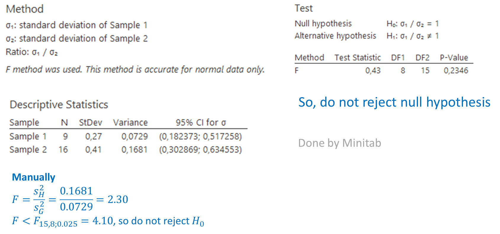
Grolsch vs. Heineken (known variances)

Some students claim that on the average a Grolsch barrel ( $\mu_G$ ) of beer contains more beer than a Heineken barrel ( $\mu_H$ ). Both brewers claim that a barrel of beer contains $50$ liters or more.
Now we have the hypotheses:

$\displaystyle{H_0: \mu_G-\mu_H=0}$ ; $\displaystyle{H_1: \mu_G-\mu_H<0}$

The students want to investigate this claim and use a sample of 9 barrels of Grolsch and 16 barrels of Heineken and find:

$\displaystyle{\overline{X}_G=49.9}$ liter and $\displaystyle{\overline{X}_H=50.1}$ .

The population standard deviations are assumed to be known:

$\sigma_G=0.4$ liter and $\sigma_H=0.3$ liter.

Now we have:

$\displaystyle{\mu_G=50$ , $\sigma_G=0.3$ , $\overline{X}_G=49.9$ , $n_G=9}$

$\displaystyle{\mu_H=50$ , $\sigma_H=0.4$ , $\overline{X}_H=50.1$ , $n_H=16}$

$\displaystyle{H_0: \mu_G-\mu_H=0}$

$\displaystyle{H_1: \mu_G-\mu_H<0}$

The significance level is $\alpha=0.05$ .
We compute the $Z$ statistic (known variances) and find:

$Z=-1.41$

The rejection region is $Z<-Z_{0.05}=-1.645$ .

The test statistic does not fall into the rejection region and thus there is insufficient evidence to reject $H_0$

Minitab Express finds the following result:

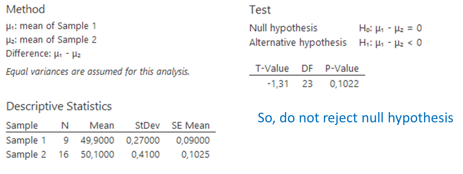
Grolsch vs. Heineken (unknown variances)

Suppose we do not know the population variances. Then we need to verify whether we may assume the variances to be equal. This test is carried out by Minitab Express and shows that we may assume the unknown variances to be equal.

Now we may use the pooled test statistic and find:

$t=-1.31$

The rejection region is:

$t<-t_{23;0.05]=-1.714$

Again, there is insufficient evidence to reject $H_0$ .

Minitab Express confirms this result:

Matched pairs

We illustrate this case by the following example.

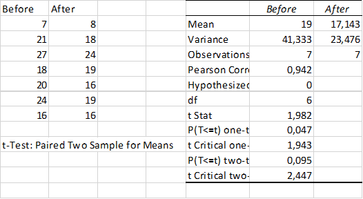
In a preliminary study to determine whether the installation of a camera designed to catch cars that go through red lights affects the number of violators, the number of red-light runners was recorded for each day of the week before and after the camera was installed.

Day	Before	After	Difference
Sunday	7	8	-1
Monday	21	18	+3
Tuesday	27	24	+3
Wednesday	18	19	-1
Thursday	20	16	+4
Friday	24	19	+5
Saturday	16	16	0
Total			13

Can we infer that the camera reduces the number of red-light runners? Obviously, the samples ‘before’ and ‘after’ are not independent. The purpose of the installation is that the number of red-light runners ‘after’ will be less than ‘before’, so:

$\mu_D=$ the difference ‘means before’ – ‘means after’

$H_0: \mu_D=0; H_1:\mu_D>0$

In this experimental design the parameter of interest is the mean of the population of differences $\mu_D=\mu_1-\mu_2$ .

The test statistic for the mean of the population differences is:

$\displaystyle{t=\frac{\overline{X}_D-\mu_D}{s_D/\sqrt{n_D}}}$

which is Student’s $t$ distributed with $n_D-1$ degrees of freedom, provided that the differences are (approximately) normally distributed.
We compute the mean of the differences: $\overline{X}_D=1.86$ and the sample standard deviation: $s_D=2.48$ . The test statistic is:

$\displaystyle{t=\frac{\overline{X}_D}{s_D/\sqrt{n_D}}=\frac{1.86}{2.48/\sqrt{7}}}=1.98$

The rejection region is $\displaystyle{t>t_{\alpha;\nu}=t_{0.05;6}=1.943}$

The test statistic falls into the rejection region, so reject $H_0$ . The installation seems to reduce the red-light runners although there is no overwhelming evidence (see also the Excel output below).

Difference between two proportions

If $x_1$ and $x_2$ are the number of successes in samples of sizes $n_1$ and $n_2$ , then:

$\displaystyle\hat{p}_1}=\frac{x_1}{n_1}}$

$\displaystyle{\hat{p}_2}=\frac{x_2}{n_2}}$

estimate the population proportions $p_1$ and $p_2$ respectively. The sampling distribution of $\displaystyle{\hat{p}_1-\hat{p}_2}$ is (approximately) normally distributed provided some requirements hold. The following formulas hold:

$\displaystyle{E(\hat{p}_1-\hat{p}_2)=\mu_{\hat{p}_1}-\mu_{\hat{p}_2}=p_1-p_2}}$

$\displaystyle{\sigma_{\hat{p}_1-\hat{p}_2}=\sqrt{\frac{p_1(1-p_1)}{n_1}+{\frac{p_2(1-p_2)}{n_2}}}$

so, the test statistic is:

$\displaystyle{Z=\frac{(\hat{p}_1-\hat{p}_2)-(p_1-p_2)}{\sqrt{\frac{p_1(1-p_1)}{n_1}+\frac{p_2(1-p_2)}{n_2}}}}$

which is (approximately) standard normally distributed.

We consider two cases:

1. $\displaystyle{H_0:p_1-p_2=0$ and 2. $H_0:p_1-p_2=D, D\neq0}$

Case 1
If $H_0: p_1-p_2=0$

then we assume $p_1=p_2$ and then we use the pooled proportion estimate:

$\displaystyle{\hat{p}=\sqrt{\frac{x_1+x_2}{n_1+n_2}}}}$

which leads to the following test statistic:

$\displaystyle{Z=\frac{\hat{p}_1-\hat{p}_2}{\sqrt{\hat{p}(1-\hat{p})(\frac{1}{n_1}+\frac{1}{n_2})}}}$

Case 2
If $H_0:p_1-p_2=D, D\neq0$

then we use the following test statistic:

$\displaystyle{Z=\frac{(\hat{p}_1-\hat{p}_2)-D}{\sqrt{\frac{\hat{p}_1(1-\hat{p}_1)}{n_1}+\frac{\hat{p}_2(1-\hat{p}_2}{n_2})}}}$

Example
Suppose:

$\displaystyle{x_1=180, n_1=904; x_2=155, n_2=1038}$

$\displaystyle{H_0:p_1-p_2=0; H_1:p_1-p_2>0; \alpha=0.05}$

$\displaystyle{\hat{p}_1=\frac{180}{904}=0.1991; \hat{p}_2=\frac{155}{1038}=0.1493}$

The pooled proportion is:

$\displaystyle{\hat{p}=\frac{180+155}{904+1038}=0.1725}$

The pooled test statistic is:

$\displaystyle{Z=\frac{\hat{p}_1-\hat{p}_2}{\sqrt{\hat{p}(1-\hat{p})(\frac{1}{n_1}+\frac{1}{n_2})}}}=$

$\displaystyle{Z=\frac{0.1991-0.1493}{\sqrt{0.1725(1-0.1725)(\frac{1}{904}+\frac{1}{1038})}}}=2.90$

The rejection region is $Z_{0.05}>1.645$

The test statistic falls into the rejection region and thus at the $5$ % significance level the null hypothesis is rejected.

Analysis Of Variance: ANOVA

Analysis of variance is a technique that allows us to compare two or more populations of interval data:

$\mu_1=\mu_2=\cdots=\mu_k$

ANOVA is an extension of the previous ‘compare means’ problems which is only for two populations.

ANOVA is a procedure which determines whether differences exist between population means. It works by analyzing the sample variances.

Independent samples are drawn from $k$ populations:

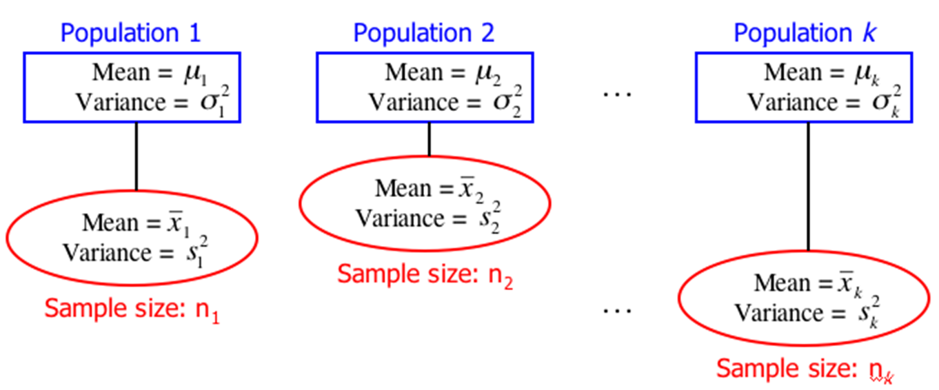
The populations are referred to as treatments (for historical reasons). $X$ is the response variable and its values are responses.

$X_{ij}$ refers to the $i^{th}$ observation (row) in the $j^{th}$ sample (column). E.g. $X_{35}$ is the $3$ ^rd observation in the $5$ ^th sample.

The grand mean $\overline{\overline{X}}$ is the mean of all observations:

$\displaystyle{\overline{\overline{X}}=\frac{\sum_{j=1}^{k}\sum_{i=1}^{n_j}X_{ij}}{n}}$

with $\displaystyle{n=n_1+n_2+\cdots+n_k}$

One-way ANOVA: Stock market

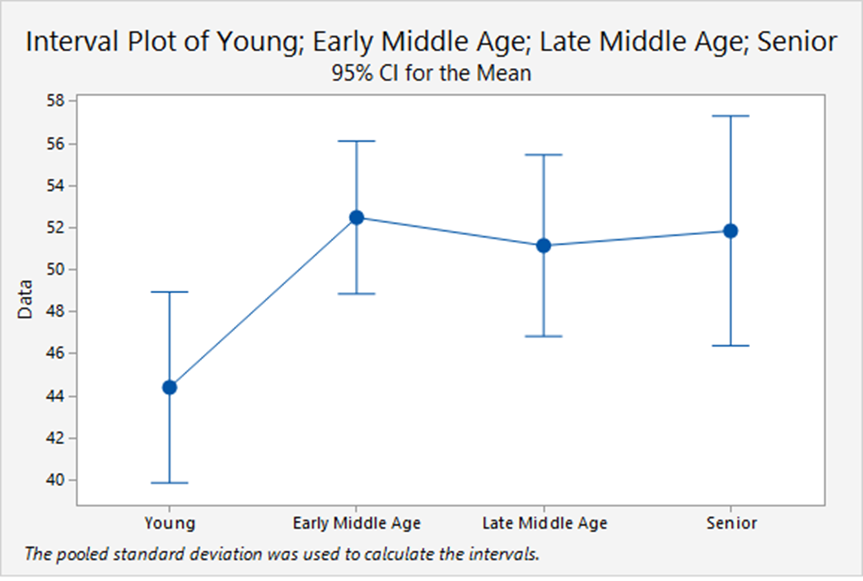
A financial analyst randomly sampled 366 American households and asked each to report the age of the head of the household and the proportion of their financial assets that are invested in the stock market.
The age categories are:

Young (Under 35);
Early middle-age (35 to 49);
Late middle-age (50 to 65);
Senior (Over 65).

The analyst was particularly interested in determining whether there are differences in stock ownership between the age groups.

The percentage $X$ of total assets invested in the stock market is the response variable; the actual percentages are the responses in this example.

Population classification criterion is called a factor.

The Age category is the factor we are interested in;
Each population is a factor level;
In this example, there are four factor levels: Young, Early middle age, Late middle age, and Senior.

The hypotheses are:

$H_0:\mu_1=\mu_2=\mu_3=\mu_4$

$H1:$ at least two means differ

Since $\mu_1=\mu_2=\mu_3=\mu_4$ is of interest to us, a statistic that measures the proximity of the sample means to each other would also be of interest.
Such a statistic exists, and is called the between-treatments variation.

The between-treatments variation is denoted $SST$ , short for “Sum of Squares for Treatments”. It is calculated as:

$\displaystyle{SST=\sum_{j=1}^{k}n_j(\overline{X}_j-\overline{\overline{X}})^2}$

If $\overline{X}_j$ are equal then $\overline{X}_j=\overline{\overline{X}}$ and $SST=0$ . A large $SST$ indicates large variations between sample means which supports $H_1$ .

A second statistic, $SSE$ (Sum of Squares for Error) measures the within-treatments variation.

$\displaystyle{SSE=\sum_{j=1}^{k}\sum_{i=1}^{n_j}(X_{ij}-\overline{X}_j)^2}$

$\displaystyle{SSE=\sum_{j=1}^{k}(n_j-1){s_j}^2}$

In the second formulation, it is easier to see that it provides a measure of the amount of variation we can expect from the random variable we have observed.

The total variation (of all observations) is:

$\displaystyle{SS$ (Total)} $\displaystyle{=\sum_{j=1}^{k}\sum_{i=1}^{n_j}(X_{ij}-\overline{\overline{X}})^2}$

We can prove:

$\displaystyle{SS$ (Total) $=SST+SSE}$

Since:

$\displaystyle{SST=\sum_{j=1}^{k}n_j(\overline{X}_j-\overline{\overline{X}})^2}$

and if:

$\displaystyle{\overline{X}_1=\overline{X}_2=\overline{X}_3=\overline{X}_4(=\overline{\overline{X}})}$

then:

$\displaystyle{SST=0}$

and our null hypothesis:

$\mu_1=\mu_2=\mu_3=\mu_4$

would be supported.

More generally, a small value of $SST$ supports the null hypothesis. A large value of $SST$ supports the alternative hypothesis. The question is, how large is “large enough”?

If we define the mean square for treatments:

$\displaystyle{MST=\frac{SST}{k-1}}$

and the mean square for error:

$\displaystyle{MSE=\frac{SSE}{n-k}}$

then the test statistic:

$\displaystyle{F=\frac{MST}{MSE}}$

has a $F$ distribution wih $k-1$ and $n-k$ degrees of freedom.

In example 14.1 (Keller) we calculated:

$MST=1247.12$

and:

$MSE=447.16$

and thus the test statistic is:

$\displaystyle{F=\frac{MST}{MSE}=\frac{1247.12}{447.16}=2.79}$

The rejection region is:

$\displaystyle{F>F_{k-1, n-k;\alpha}=F_{3,362;0.05}=2.62}$

The test statistic falls into the rejection region, so we reject $H_0$ .
The following plot shows the details.

and Excel gives the following results. Note the relation between $F,F_{crit}$ and the $p$ -value.

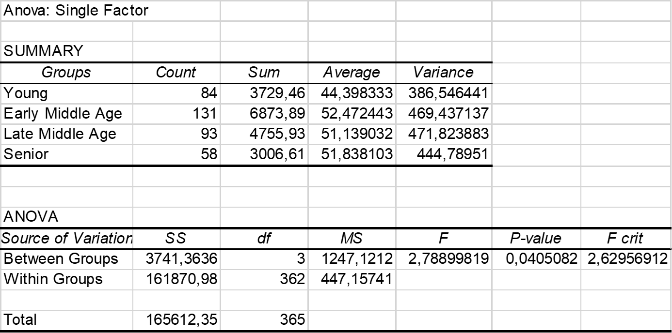
In general, the results of ANOVA are usually reported in an ANOVA table as can be seen in the Excel output.

Source of Variation	Degrees of freedom	Sum of Squares	Mean Square
Treatments	k–1	SST	MST=SST/(k–1)
Error	n–k	SSE	MSE=SSE/(n–k)
Total	n–1	SS(Total)

One question has to be answered. In this case, what do we need ANOVA for? Why not test every pair of means? For example, say $k=6$ . Then there are $\displaystyle{\binom{6}{2}=15}$ different pairs of means,

1&2 1&3 1&4 1&5 1&6
2&3 2&4 2&5 2&6
3&4 3&5 3&6
4&5 4&6
5&6

If we test each pair with $\alpha=0.05$ we increase the probability of making a Type I error. If there are no differences then the probability of making at least one Type I error is

$1-(0.95)^{15}=1-0.463 =0.537$