(Keller 7, 8, 9)
Probability distributions
(Keller 7, 8)
A probability distribution is a table, formula or graph that describes the values of a random variable and the probability associated with these values. Since a random variable can be either discrete or continuous we have two types of probability distributions: discrete and continuous probability distributions.
An example of a formula as distribution function is the following continuous normal distribution function.

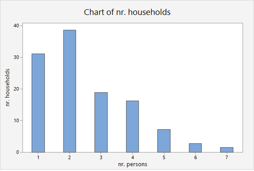
An example of a table is the following table which describes a discrete distribution function.
| Number of persons | Number of households |
|---|---|
| 1 | 31.1 |
| 2 | 38.6 |
| 3 | 18.8 |
| 4 | 16.2 |
| 5 | 7.2 |
| 6 | 2.7 |
| 7 or more | 1.4 |
| Total | 116.0 |
Discrete probability distributions
(Keller 7)
The following requirements hold for the the probability  :
:
 for all

There is a relation between the relative frequency diagram and the discrete probability function.
Distribution of the households
The probability distributions can be estimated from relative frequencies.
 is a discrete variable, the number of persons in a household.
| X | # households millions | P(x) |
| 1 | 31.1 | .268 |
| 2 | 38.6 | .333 |
| 3 | 18.8 | .162 |
| 4 | 16.2 | .140 |
| 5 | 7.2 | .062 |
| 6 | 2.7 | .023 |
| 7 or more | 1.4 | .012 |
| Total | 116.0 | 1.00 |
is the discrete probability distribution of the number of persons in a household.
We have:  , etc.
Also we can compute 
Population mean E(X)
(Keller 7)
The population mean  is the weighted average of all values of . The weights are the probabilities.
 is called the expected value of and is defined by the following formula.

Example: a dice
What is the mean of throws of a fair dice.?
 for all
and thus:
Population variance V(X)
(Keller 7)
The population variance  is calculated similarly. It is the weighted average of the squared deviations from the mean . The weights are the probabilities. It is defined by the following formula:

Example: distribution of households


The standard deviation is  .
.
Covariance of two discrete variables
The covariance of two discrete variables and  is defined as:

 is the joint probability distribution of the random variables and :
  and
and  .
.
Note. We also write  .
.
Laws of E(X) and V(X)
(Keller 7)


These formulas can easily be derived from the definition of


These formulas can easily be derived from the definition of 
For example: 
Laws about sum of variables
(Keller, p. 234 ( and
and  are two random variables)


If and are independent then  and thus:

Example
If and are independent then (because  and
and  :
:

Coefficient of correlation
The coefficient of correlation is defined as the covariance divided by the standard deviations of the variables.
The population coefficient of correlation is:

The sample coefficient of correlation is:

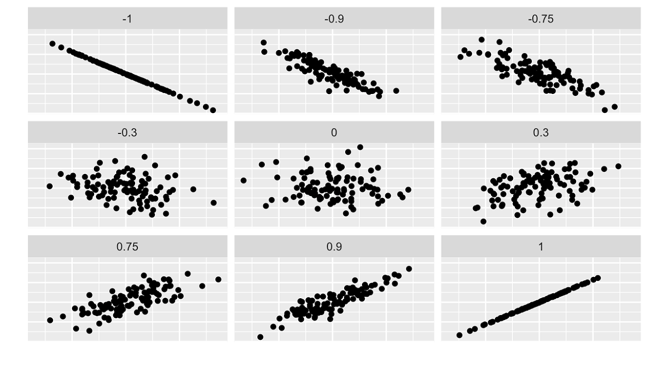
The coefficient of correlation answers the question: how strong is the association between and ?
The advantage of the coefficient of correlation over the covariance is that it has a fixed range from  to
to  (proven by Mathematics). If the two variables are very strongly and positively related, the coefficient value is close to (strong positive linear relationship). If the two variables are very strongly and negatively related, the coefficient value is close to (strong negative linear relationship). No straight linear relationship is indicated by a coefficient close to 0.
The following graphs depict the relations of and for various coefficients of correlation, varying from to .
Binomial distribution
(Keller 7)
The binomial distribution is the probability distribution that results from doing a binomial experiment. Binomial experiments have the following properties:
- There are a fixed number of trials, represented as

- Each trial has two possible outcomes, success or failure
 ;
;  for all trials
- The trials are independent, meaning that the outcome of one trial does not affect the outcomes of any other trials.
The binomial random variable counts the number of successes in trials of the binomial experiment.
(e.g. s s f s f f f s f s s f s shows  trials and
  successes).
To calculate the probability associated with each value we use combinatorics:
 for
for 
Example
A quiz consists of  independent multiple-choice questions (
 ). Each question has
  possible answers, only one of which is correct (
 ). You choose to guess the answer to each question. is the number of correct guesses
  . The probability that you will have a score
  is:
is:

{ is called factorial
  ;
;  ;
;  )
)
Mean and variance
(Keller 7)
The mean, variance and standard deviation of a binomial random are variable (can be derived mathematically):

 and thus:

Continuous random variables
(Keller 8)
Unlike a discrete random variable, a continuous random variable is one that assumes an uncountable number of values. We cannot list the possible values because there is an infinite number of them. Because there is an infinite number of values, the probability of each individual value is  . So, the probability that a man has a height of exactly 180 cm is:
![P(X=180)=\lim_{\epsilon\to0}[P(180+\epsilon)-P(180-\epsilon)]=0](https://4mules.nl/wp-content/ql-cache/quicklatex.com-7b8334fb77df400000d3e462898b216a_l3.png "Rendered by QuickLaTeX.com")
Pobability density functions
{Keller 8)
A function  is called a probability density function (over the range
  ) if it meets the following requirements:
 for all
 ![x\in[a,b]](https://4mules.nl/wp-content/ql-cache/quicklatex.com-078c131b584569a7e42af1ff12296275_l3.png "Rendered by QuickLaTeX.com")
The total area between curve and -axis is:

For the interval [a, b] we may also take  , as is the case in e.g. the normal distribution.
The normal density function
(Keller 8)
The normal distribution is the most important of all probability distributions. The probability density function  of a normal random variable is given by:
 for
for 
The graph is bell-shaped and symmetrical around the mean . This density function is also denoted by  or
or  .
.
The normal distribution function is defined by:

Therefore, the probability  equals
  .
.
This infinite integral cannot be computed analytically (pen and paper), therefore we need a table or a computer can do the job.
Standard normal distribution
(Keller 8)
A normal density function with mean  and standard deviation
  is called the standard normal density.
 for
for 
Any normal distribution can be converted to a standard normal distribution, see below. The standard normal distribution is also denoted by  .
.
Any (normal) variable can be converted to a new (normal) variable  :
:

with the following properties:

 .
.
Thus, if

then
 .
.
Example
Suppose the demand is a normally distributed variable with mean  and standard deviation
  and we want to compute
  . Then:


 .
.
The answer can be found in Table 3 of Appendix B9 of Keller, or by Excel.
Other continuous distributions
There are three other continuous distributions which will be used later.
 distribution (also called Student's distribution)
 (ci-squared) distribution)
 distribution
Sampling distributions
(Keller 9)
A sample of size is just one of many possible samples of size . If  is the population size and the sample size (≪) then the number of possible different samples equals
  .
.
They are usually very large, e.g.: 
Most samples have (different) random statistics, e.g.  or
or  .
.
These sample statistics have a probability distribution, the so-called sampling distribution.
Some mathematics
 and are sample statistics. Let us derive the distribution function of . We know that
  and
and  . Then:


So, for ther random variable it holds:  and
and 
Earlier we defined for any random variable :

and thus for the random variable we get:

Central Limit Theorem
(Keller 7, 8, 9)
The sampling distribution of the means of random samples drawn from any population is approximately normal for a sufficiently large sample size . The larger the sample size, the more closely the sampling distribution of  will resemble a normal distribution.
If the distribution of the population is normal, then is normally distributed for all sample sizes . If the population is non-normal, then is approximately normal only for larger values of . In most practical situations, a sample size of  may be sufficiently large to allow us to use the normal distribution as an approximation for the sampling distribution of .
Verify Central Limit Theorem
(Keller 9)
The following is a program in pseudo code.
- Take a first sample of size of a uniform distribution and compute its sample mean
 ;
; - Repeat this
 times and thus get
  sample means
  . Also these means are random variables.
 - According to the Central Limit Theorem these random means should be (approximately) normally distributed.
- Verify this graphically by drawing a histogram.
- Verify this by applying a normality test (e.g. Anderson-Darling).
- Repeat 1-5 for
 and notice the differences.
The actual program is executed by the programming language but any programming language can do the job. Thc code of the R program is as follows:
# Suppose x has a uniform distribution
# n is the sample size, preferably n = 30
n <- 30
# k is the number of such sample means, sufficiently large, e.g. k = 5000
k <- 5000
# According to the Central Limit Theorem
# the k sample means should approximate a normal distribution
z <- numeric(k) # z is a vector with k elements and will contain all k sample means
for (j in 1:k) (z[j] <- mean(runif(n))) # compute the mean of each uniform sample
# show the histogram of these means
hist(z)
# and find out whether the distribution of means is normal
# which is approximately true for n ≥ 30
ad.test(z) # Anderson-Darling test
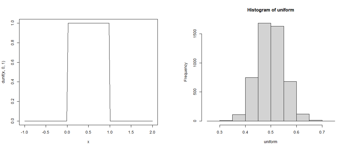
The result is as follows.
The left graphs represents a unoform distribution on ![[0,1]](https://4mules.nl/wp-content/ql-cache/quicklatex.com-4ddc1168784a8b723604919df78ae658_l3.png "Rendered by QuickLaTeX.com") ; the right graph depicts a histogram of sample means which is rather good approximation of a normal distribution.
; the right graph depicts a histogram of sample means which is rather good approximation of a normal distribution.
Using the standard normal distribution
(Keller 9)
Suppose the population random variable is normally distributed with  and
and  .
.
We take a sample of size  drawn from the population. The sample mean is denoted by
  . We want to compute
  .
.
We know:
is normally distributed, therefore so will be .
 and
and 
 Let op: fout in formule.

The answer can be found in Table 3 of Appendix B9 of Keller.
The difference of two means
(Keller 9)
Consider the sampling distribution of the difference  of two sample means.
If the random samples are drawn from each of two independent normally distributed populations, then will be normally distributed as well with:


Let op: fout in formule.
If two populations are not both normally distributed, and the sample sizes are large enough ( ), then in most cases the distribution of is approximately normal (see the Central Limit Theorem).
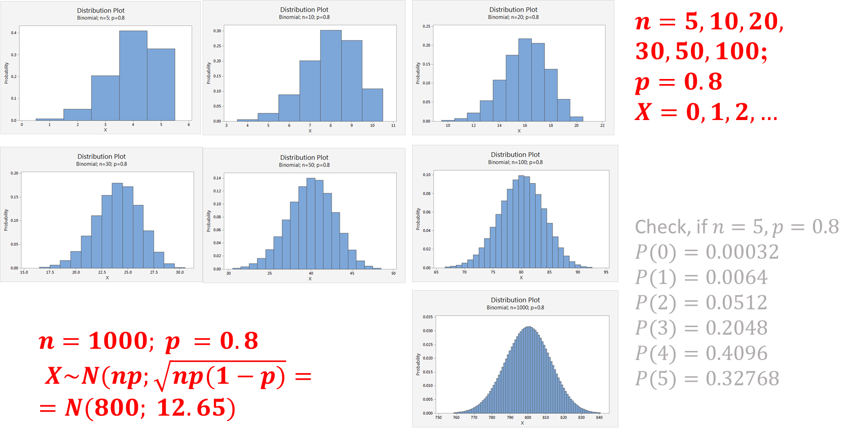
Normal approximation to Binomial
See the following example: a binomial distribution with  and
and  superimposed by a normal distribution (
 and
and  ).
).
The graph shows  and the graph of a
  distribution. See the formulas of the probabilities of a binomial distribution.
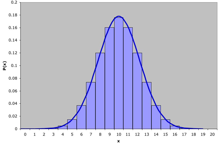
The normal approximation to binomial works best when the number of experiments is large and the probability of succes  is close to
  .
.
For the approximation to provide acceptable results two conditions should be met:
 and
and 
The following graph shows the approximations witp  and various values of .
Example
For a binomial distribution ( we find (using Excel):
 .
.
For a normal distribution ( ) we find:
 (continuity correction).
Distribution of a sample proportion
The estimator of a population proportion of successes is the sample proportion. That is, we count the number of successes in a sample of size and compute:

is the number of successes, is the sample size.
Note that the random variable has binomial distribution.
Using the laws of expected value and variance, we can determine the mean, variance and standard deviation. Sample proportions can be standardized to a standard normal distribution using the formula:
and thus 
Note.
Binomial disribution: 


and thus:

Example
In the last election a state representative received  % of the votes (so
  ; this can be considered as a population parameter!)
One year after the election the representative organized a survey that asked a random sample of  people whether they would vote for him in the next election.
If we assume that his popularity has not changed what is the probability that more than half of the sample would vote for him?
The number of respondents who would vote for the representative is a binomial random variable with and and we want to determine the probability that the sample proportion is greater than  %, That is, we want to compute
  .
.
From the foregoing we know that the sample proportion  is approximately normally distributed with mean and standard deviation
Thus we compute:


If we assume that the level of support remains at % the probability that more than half the sample of  people would vote for the representative is
  %.
%.