We already used the  test for hypothesis testing of variances. These tests are also used for goodness-of-fit tests and testing contingency (cross) tables.
We will explain both applications in a number of examples.
Goodness-of-fit test
The goodness-of-fit test is applied to data produced by a multinomial experiment which is a generalization of a binomial experiment and is used to describe one population of data. It consists of a fixed number of  trials. Each trial can have one of
  outcomes, called cells. Each probability
  remains constant. Our usual notion of probabilities holds, namely:

and each trial is independent of the other trials.
We test whether there is sufficient evidence to reject a specified set of values for .
To illustrate this, our null hypothesis is:

where
 are the values we want to test, and:
 At least one is not equal to its specified value.
Market shares companies A and B
Two companies, A and B have the following market shares:
A: 45%, B: 40%, Others: 15%.
After a marketing campaign a random sample of 200 customers showed that:
102 customers preferred A;
82 preferred B; and
16 preferred other companies.
Can we infer at the 5% significance level that customer preferences have changed from their levels before the advertising campaigns were launched?
We compare the market share before and after the advertising campaign to see if there is a difference. We hypothesize values for the parameters equal to the before-market share. That is,

at least one is not equal to its specified value.
If the null hypothesis is true, we would expect the number of customers selecting brand A, brand B, and others:
 ;
; 
 ;
; 
 ;
; 
 expected number of customers.
 observed number of customers (marketing analysis)
The  (chi-squared) goodness-of-fit test statistic is given by:

Note.
If  then
then 
If  then
then 
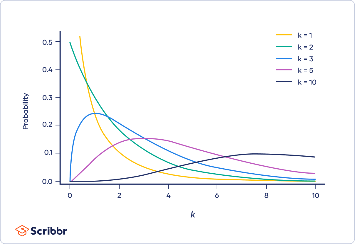
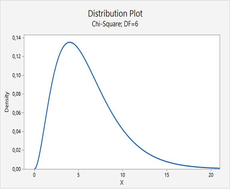
This statistic is (approximately) distributed with  degrees of freedom, provided the sample size is large. The rejection region is:
  .
.
The rejection region is  .
.
The test statistic is  which falls into the rejection region, so we reject
  in favor of
  .
.
 distributions
Conclusion: there is sufficient evidence to infer that the proportions have changed since the advertising campaigns were implemented.
There are some requirements for the goodness-of-fit test. First, in order to use this technique, the sample size must be large enough so that the expected value for each cell is 5 or more. If the expected frequency in a cell is less than five, it would be better to combine that cell with other cells to satisfy the condition.
Contingency (cross) tables
Again we explain this topic by an example.
An MBA program was experiencing problems scheduling their courses. The demand for the program's optional courses and majors was quite variable from one year to the next. An investigator believed that the problem may be that the undergraduate degree affects the choice of a major.
Therefore, he took a random sample of last year's MBA students and recorded the undergraduate degree and the major selected in the graduate program. The undergraduate degrees were BA (Bachelor of Arts), BEng (Bachelor of Engineering) , BBA (Bachelor of Business Administration), and others.
There are three possible majors for the MBA students, accounting, finance, and marketing. Can he conclude at the 5% significance level that the undergraduate degree affects the choice of the major? In fact, are the undergraduate degree and the majors independent?

 MBA major and Undergraduate degree are independent; They are not independent.
Based on this table we construct a table with the observed and expected values.
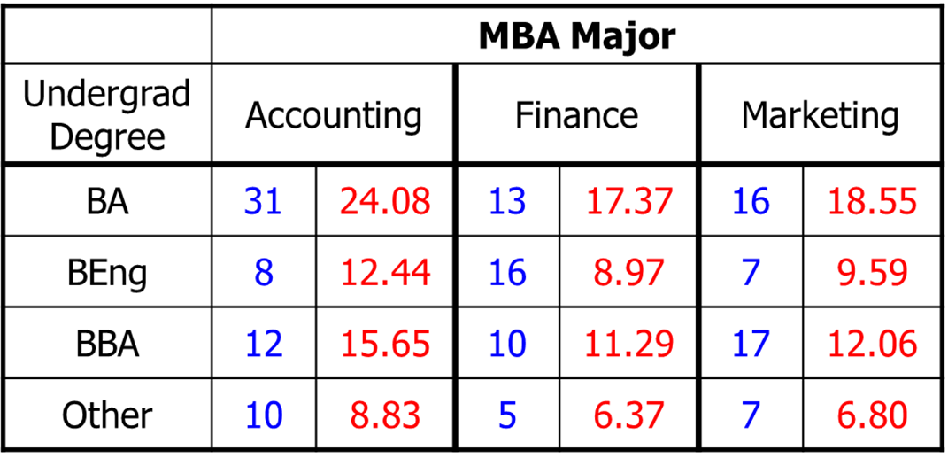
Blue: Observed values
Red: Expected values
How do we compute the expected values? As an example we take the cell (BA, Accounting):
 (BA, Accounting)
The test statistic is:

The rejection region is:

falls into the rejection region and thus reject .
Of course, Excel gives the same results.
 |  |  | |
| 31 | 24,08 | 1,99 | |
| 13 | 17,37 | 1,10 | |
| 16 | 18,55 | 0,35 | |
| 8 | 12,44 | 1,58 | |
| 16 | 8,97 | 5,51 | |
| 7 | 9,59 | 0,70 | |
| 12 | 15,65 | 0,85 | |
| 10 | 11,29 | 0,15 | |
| 17 | 12,06 | 2,02 | |
| 10 | 8,83 | 0,16 | |
| 5 | 6,37 | 0,29 | |
| 7 | 6,80 | 0,01 | |
| Total | 14,71 | ||
| Rej. Level | 12,59 | ||
| So, reject H0 |
Coefficient of correlation
Sometimes we want to know whether there is a linear relationship between two population variables. For this we use the population coefficient of correlation  :
:
 :
:
Recall: ![\displaystyle{\rho\in{[-1,+1]}}](https://4mules.nl/wp-content/ql-cache/quicklatex.com-928821e1d1e4827b85541d023db9bb13_l3.png "Rendered by QuickLaTeX.com")
 minimal negative relation
 maximal positive relation
 no relation
The population coefficient of correlation is denoted by . We estimate its value from sample data with the sample coefficient of correlation:

The test statistic for testing  is:
is:

If  or
or  or
or 
The rejection region is:
 or
or  or
or 
In Keller (p. 655) an example is used giving the data of the relation between the price and odometer readings of trade-in cars. Are these data correlated?
The correlation is computed and we define the null and alternative hypotheses. We get:

The test statistic is:

The rejection region is:

So, there is overwhelming evidence that odometer readings and price are correlated. We reject the null hypothesis.